Image Arithmetic
We know that images are nothing but matrices. This raises an important and interesting question. If we can carry out arithmetic operations on matrices, can we carry them out on images as well? The answer is a bit tricky. We can carry out the following operations on images:
- Adding and subtracting two images
- Adding and subtracting a constant value to/from image
- Multiplying a constant value by an image
We can, of course, multiply two images if we can assume they're matrices, but in terms of images, multiplying two images does not make much sense, unless it's carried out pixel-wise.
Let's look at these operations, one by one.
Image Addition
We know that an image is made up of pixels and that the color of a pixel is decided by the pixel value. So, when we talk about adding a constant to an image, we mean adding a constant to the pixel values of the image. While it might seem a very simple task, there is a small concept that needs to be discussed properly. We have already said that, usually, the pixel values in images are represented using unsigned 8-bit integers, and that's why the range of pixel values is from 0 to 255. Now, imagine that you want to add the value 200 to an image, that is, to all the pixels of the image. If we have a pixel value of 220 in the image, the new value will become 220 + 200 = 420. But since this value lies outside of the range (0-255), two things can happen:
- The value will be clipped to a maximum value. This means that 420 will be revised to 255.
- The value will follow a cyclic order or a modulo operation. A modulo operation means that you want to find the remainder obtained after dividing one value by another value. We are looking at division by 255 here (the maximum value in the range). That's why 420 will become 165 (the remainder that's obtained after dividing 420 by 255).
Notice how the results obtained in both approaches are different. The first approach, which is also the recommended approach, uses OpenCV's cv2.add function. The usage of the cv2.add function is as follows:
dst = cv2.add(src1, src2)
The second approach uses NumPy while adding two images. The NumPy approach is as follows:
dst = src1 + src2
src1 refers to the first image that we are trying to add to the second image (src2). This gives the resultant image (dst) as the output. Either of these approaches can be used to add two images. The interesting part, as we will see shortly in the next exercise, is that when we add a constant value to an image using OpenCV, by default, that value gets added to the first channel of the image. Since we already know that images in OpenCV are represented in BGR mode, the value gets added to the blue channel, giving the image a more bluish tone. On the other hand, in the NumPy approach, the value is automatically broadcasted in such a manner that the value is added to every channel.
Let's compare both approaches with the help of an exercise.
Exercise 2.04: Performing Image Addition
In this exercise, we will learn how to add a constant value to an image and the approaches to carry out the task. We will be working on the following image. First, we will add a constant value to the image using the cv2.add function and then compare the output obtained with the output obtained by adding the constant value using NumPy:
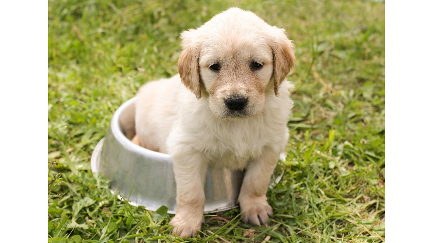
Figure 2.27: Image of a Golden Retriever puppy
Note
This image can be found at https://packt.live/2ZnspEU.
Follow these steps to complete this exercise:
- Create a new notebook –
Exercise2.04.ipynb. We will be writing our code in this notebook. - Let's import the libraries we will be using and also write the magic command:
# Import libraries
import cv2
import numpy as np
import matplotlib.pyplot as plt
%matplotlib inline
- Read the image. The code for this is as follows:
Note
Before proceeding, be sure to change the path to the image (highlighted) based on where the image is saved in your system.
# Read image img = cv2.imread("../data/puppy.jpg") - Display the image using Matplotlib:
# Display image
plt.imshow(img[:,:,::-1])
plt.show()
The output is as follows. The X and Y axes refer to the width and height of the image, respectively:

Figure 2.28: Image of a Golden Retriever puppy
- First, try adding the value 100 to the image using NumPy:
# Add 100 to the image
numpyImg = img+100
- Display the image, as follows:
# Display image
plt.imshow(numpyImg[:,:,::-1])
plt.show()
The output is as follows. The X and Y axes refer to the width and height of the image, respectively:

Figure 2.29: Result obtained by adding 100 to the image using NumPy
Notice how adding the value 100 has distorted the image severely. This is because of the modulo operation being performed by NumPy on the new pixel values. This should also give you an idea of why NumPy's approach is not the recommended approach to use while dealing with adding a constant value to an image.
- Try doing the same using OpenCV:
# Using OpenCV
opencvImg = cv2.add(img,100)
- Display the image, as follows:
# Display image
plt.imshow(opencvImg[:,:,::-1])
plt.show()
The output is as follows. The X and Y axes refer to the width and height of the image, respectively:

Figure 2.30: Result obtained by adding 100 to the image using OpenCV
As shown in the preceding figure, there is an increased blue tone to the image. This is because the value 100 has only been added to the first channel of the image, which is the blue channel.
- Fix this by adding an image to an image instead of adding a value to an image. Check the shape, as follows:
img.shape
The output is
(924, 1280, 3). - Now, create an image that's the same shape as the original image that has a fixed pixel value of 100. We are doing this because we want to add the value 100 to every channel of the original image:
nparr = np.ones((924,1280,3),dtype=np.uint8) * 100
- Add
nparrto the image and visualize the result:opencvImg = cv2.add(img,nparr) # Display image plt.imshow(opencvImg[:,:,::-1]) plt.show()
The output is as follows. The X and Y axes refer to the width and height of the image, respectively:

Figure 2.31: Result obtained by adding an image to another image
- When the same image is added using OpenCV, we notice that the results that are obtained are the same as they were for NumPy:
npImg = img + nparr
# Display image
plt.imshow(npImg[:,:,::-1])
plt.show()
The output is as follows. The X and Y axes refer to the width and height of the image, respectively:

Figure 2.32: New results obtained
The most interesting point to note from the results is that adding a value to an image using OpenCV results in increased brightness of the image. You can try subtracting a value (or adding a negative value) and see whether the reverse also true.
In this exercise, we added a constant value to an image and compared the outputs obtained by using the cv2.add function and by using NumPy's addition operator (+). We also saw that while using the cv2.add function, the value was added to the blue channel and that it can be fixed by creating an image that's the same shape as the input image, with all the pixels of the value equal to the constant value we want to add to the image.
Note
To access the source code for this specific section, please refer to https://packt.live/2BUOUsV.
In this section, we saw how to perform image addition using NumPy and OpenCV's cv2.add function. Next, let's learn how to multiply an image with a constant value.
Image Multiplication
Image multiplication is very similar to image addition and can be carried out using OpenCV's cv2.multiply function (recommended) or NumPy. OpenCV's function is recommended because of the same reason as we saw for cv2.add in the previous section.
We can use the cv2.multiply function as follows:
dst = cv2.Mul(src1, src2)
Here, src1 and src2 refer to the two images we are trying to multiply and dst refers to the output image obtained by multiplication.
We already know that multiplication is nothing but repetitive addition. Since we saw that image addition had an effect of increasing the brightness of an image, image multiplication will have the same effect. The difference here is that the effect will be manifold. Image addition is typically used when we want to make minute modifications in brightness. Let's directly see how to use these functions with the help of an exercise.
Exercise 2.05: Image Multiplication
In this exercise, we will learn how to use OpenCV and NumPy to multiply a constant value with an image and how to multiply two images.
Note
The image used in this exercise can be found at https://packt.live/2ZnspEU.
Follow these steps to complete this exercise:
- Create a new notebook –
Exercise2.05.ipynb. We will be writing our code in this notebook. - First, let's import the necessary modules:
# Import libraries
import cv2
import numpy as np
import matplotlib.pyplot as plt
%matplotlib inline
- Next, read the image of the puppy.
Note
Before proceeding, be sure to change the path to the image (highlighted) based on where the image is saved in your system.
The code for this is as follows:
# Read image img = cv2.imread("../data/puppy.jpg") - Display the output using Matplotlib, as follows:
# Display image
plt.imshow(img[:,:,::-1])
plt.show()
The output is as follows. The X and Y axes refer to the width and height of the image, respectively:

Figure 2.33: Image of a Golden Retriever puppy
- Multiply the image by
2using thecv2.multiplyfunction:cvImg = cv2.multiply(img,2)
- Display the image, as follows:
plt.imshow(cvImg[:,:,::-1])
plt.show()
The output is as follows. The X and Y axes refer to the width and height of the image, respectively:

Figure 2.34: Result obtained by multiplying the image by 2 using OpenCV
Can you think of why you obtained a high blue tone in the output image? You can use the explanation given for image addition in the previous exercise as a reference.
- Try to multiply the image using NumPy:
npImg = img*2
- Display the image, as follows:
plt.imshow(npImg[:,:,::-1])
plt.show()
The output is as follows. The X and Y axes refer to the width and height of the image, respectively:

Figure 2.35: Result obtained by multiplying the image by 2 using NumPy
- Print the shape of the image, as follows:
img.shape
The shape is
(924, 1280, 3). - Now, let's create a new array filled with 2s that's the same shape as the original image:
nparr = np.ones((924,1280,3),dtype=np.uint8) * 2
- Now, we will use this new array for multiplication purposes and compare the results that are obtained:
cvImg = cv2.multiply(img,nparr)
plt.imshow(cvImg[:,:,::-1])
plt.show()
The output is as follows. The X and Y axes refer to the width and height of the image, respectively:

Figure 2.36: Result obtained by multiplying two images using OpenCV
Note
To access the source code for this specific section, please refer to https://packt.live/2BRos3p.
We know that multiplication is nothing but repetitive addition, so it makes sense to obtain a brighter image using multiplication since we obtained a brighter image using addition as well.
So far, we've discussed geometric transformations and image arithmetic. Now, let's move on to a slightly more advanced topic regarding performing bitwise operations on images. Before we discuss that, let's have a look at binary images.