Geometric Transformations
Often, during image processing, the geometry of the image (such as the width and height of the image) needs to be transformed. This process is called geometric transformation. As we saw in the Images in OpenCV section of Chapter 1, Basics of Image Processing, images are nothing but matrices, so we can use a more mathematical approach to understand these topics.
Since images are matrices, if we apply an operation to the images (matrices) and we end up with another matrix, we call this a transformation. This basic idea will be used extensively to understand and apply various kinds of geometric transformations.
Here are the geometric transformations that we are going to discuss in this chapter:
- Translation
- Rotation
- Image scaling or resizing
- Affine transformation
- Perspective transformation
While discussing image scaling, we will also discuss image cropping. which isn't actually a geometric transformation, though it is commonly used along with resizing.
First, we will go over image translation, where we will discuss moving an image in a specified direction.
Image Translation
Image translation is also referred to as shifting an image. In this transformation, our basic intention is to move an image along a line. Take a look at the following figure:
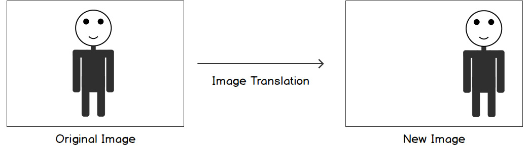
Figure 2.2: Image translation
For example, if we consider the following figure, we are shifting the human sketch to the right. We can shift an image in both the X and Y directions, as well as separately. What we are doing in this process is shifting every pixel's location in the image in a certain direction. Consider the following figure:
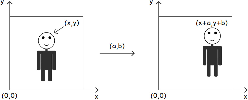
Figure 2.3: Pixel view of image translation
Using the preceding figure as reference, we can represent image translation with the following matrix equation:

Figure 2.4: Representation of an image matrix
In the preceding equation, x' and y' represent the new coordinates of a point/pixel after it has been shifted by a units in the x direction and b units in the y direction.
Note
Even though we have discussed image translation, it is very rarely used in image processing. It is usually combined with other transformations to create a more complex transformation. We will be studying this general class of transformations in the Affine Transformations section.
Now that we have discussed the theory of image translation, let's understand how translation can be performed using NumPy. We stated that images are nothing but NumPy arrays while using them in OpenCV in Python. Similarly, geometric transformations are just matrix multiplications. We also saw how image translation can be represented using a matrix equation. In terms of matrix multiplication, the same image equation can be written as a NumPy array:
M = np.array([[1,0,a],[0,1,b],[0,0,1])
If you look carefully, you will notice that the first two columns of this matrix form an identity matrix ([[1,0],[0,1]]). This signifies that even though we are transforming the image, the image dimensions (width and height) will stay the same. The last column is made up of a and b, which signifies that the image has been shifted by a units in the x direction and b units in the y direction. The last row, - [0,0,1], is only used to make the matrix, M, a square matrix – a matrix with the same number of rows and columns. Now that we have the matrix for image translation with us, whenever we want to shift an image, all we need to do is multiply the image, let's say, img (as a NumPy array), with the array, M. This can be performed as follows:
output = M@img
Here, output is the output that's obtained after image translation.
Note that in the preceding code, it's assumed that every point that we want to shift represents a column in the matrix, that is, img. Moreover, usually, an extra row full of ones is also added in the img matrix. That's simply to make sure that that matrix multiplication can be carried out. To understand it, let's understand the dimensions of the matrix, M. It has three rows and three columns. For the matrix multiplication of M and img to be carried out, img should have the same number of rows as the number of columns in matrix M, that is, three.
Now, we also know that a point is represented as a column in the img matrix. We already have the x coordinate of the point in the first row and the y coordinate of the point in the second row of the img matrix. To make sure that we have three rows in the img matrix, we add 1 in the third row.
For example, point [2,3] will be presented as [[2],[3],[1]], that is, 2 is present in the first row, 3 is present in the second row. and 1 is present in the third row.
Similarly, if we want to represent two points – [2,3] and [1,0] – they will be represented as [[2,1],[3,0],[1,1]]; that is, the x coordinates of both points (2 and 1) are present in the first row, the y coordinates (3 and 0) are present in the second row, and the third row is made up of 1s.
Let's understand this better with the help of an exercise.
Exercise 2.01: Translation Using NumPy
In this exercise, we will carry out the geometric transformation known as translation using NumPy. We will be using the translation matrix that we looked at earlier to carry out the translation. We will be shifting 3 points by 2 units in the x direction and 3 units in the y direction. Let's get started:
- Create a new Jupyter Notebook –
Exercise2.01.ipynb. We will be writing our code in this notebook. - First, let's import the NumPy module:
# Import modules
import numpy as np
- Next, we will specify the three points that we want to shift –
[2,3], [0,0], and [1,2]. Just as we saw previously, the points will be represented as follows:# Specify the 3 points that we want to translate points = np.array([[2,0,1], [3,0,2], [1,1,1]])
Note how the
xcoordinates (2, 0, and 1) make up the first row, theycoordinates (3, 0, and 2) make up the second row, and the third row has only 1s. - Let's print the
pointsmatrix:print(points)
The output is as follows:
[[2 0 1]
 [3 0 2]
 [1 1 1]]
- Next, let's manually calculate the coordinates of these points after translation:
# Output points - using manual calculation
outPoints = np.array([[2 + 2, 0 + 2, 1 + 2],
            [3 + 3, 0 + 3, 2 + 3],
            [1, 1, 1]])
- Let's also print the
outPointsmatrix:print(outPoints)
The output is as follows:
[[4 2 3]
 [6 3 5]
 [1 1 1]]
- We need to shift these points by
2units in thexdirection and3units in theydirection:# Move by 2 units along x direction a = 2 # Move by 3 units along y direction b = 3
- Next, we will specify the translation matrix, as we saw previously:
# Translation matrix
M = np.array([[1,0,a],[0,1,b],[0,0,1]])
- Now, we can print the translation matrix:
print(M)
The output is as follows:
[[1 0 2]
 [0 1 3]
 [0 0 1]]
- Now, we can perform the translation using matrix multiplication:
# Perform translation using NumPy
output = M@points
- Finally, we can display the output points by printing them:
print(output)
The output is as follows:
[[4 2 3]
 [6 3 5]
 [1 1 1]]
Notice how the output points obtained using NumPy and using manual calculation match perfectly. In this exercise, we shifted the given points using manual calculation, as well as using matrix multiplication. We also saw how we can carry out matrix multiplication using the NumPy module in Python. The key point to focus on here is that transition is nothing but a matrix operation, just as we discussed previously at the beginning of the Geometric Transformations section.
Note
To access the source code for this specific section, please refer to https://packt.live/3eQdjhR.
So far, we've discussed moving an image along a direction. Next, let's discuss rotating an image around a specified point at a given angle.
Image Rotation
Image rotation, as the name suggests, involves rotating an image around a point at a specified angle. The most common notation is to specify the angle as positive if it's anti-clockwise and negative if it's specified in the clockwise direction. We will assume angles in a non-clockwise direction are positive. Let's see whether we can derive the matrix equation for this. Let's consider the case shown in the following diagram: w and h refer to the height and width of an image, respectively. The image is rotated about the origin (0,0) at an angle, alpha (α), in an anti-clockwise direction:
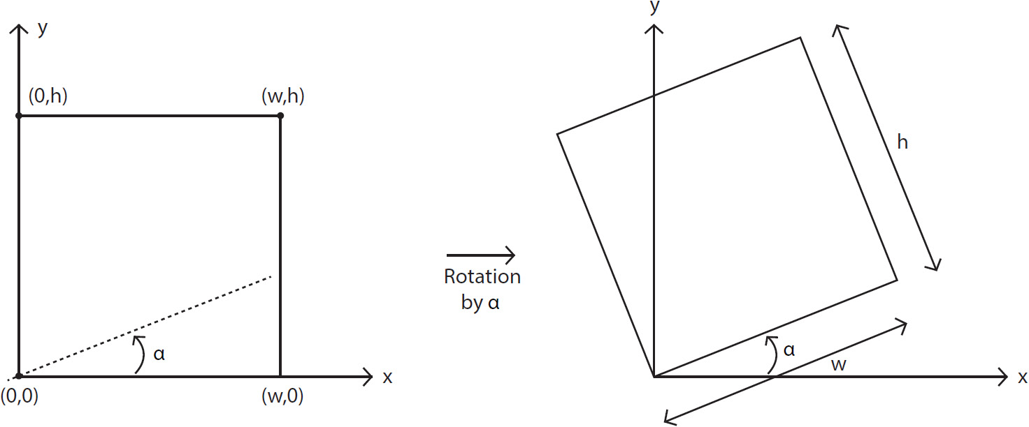
Figure 2.5: Image rotation
One thing that we can note very clearly here is that the distance between a point and the origin stays the same, even after rotation. We will be using this point when deriving the rotation matrix.
We can divide the entire problem into two parts:
- Finding the rotation matrix
- Finding the size of the new image
Finding the Rotation Matrix
Let's consider a point, P(x,y), which, after rotation by angle β around the origin, O(0,0), is transformed into P'(x',y'). Let's also assume the distance between point P and origin O is r:
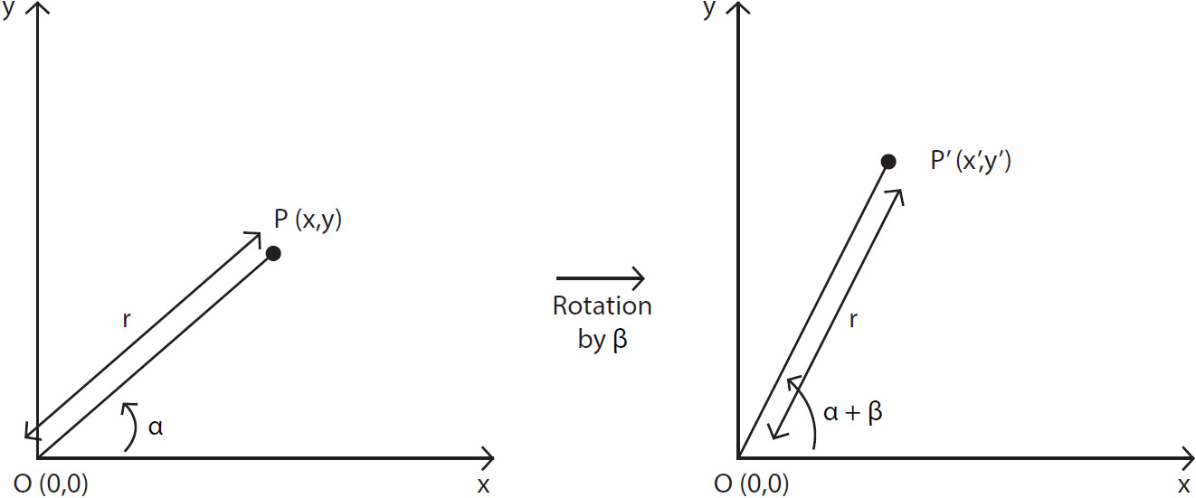
Figure 2.6: Point rotation
In the following equation, we have used the distance formula to obtain the distance between P and O:

Figure 2.7: Distance formula
Since we know that this distance will stay the same, even after rotation, we can write the following equation:

Figure 2.8: Distance formula after rotation
Let's assume that the P(x,y) point makes an angle, α, with the X-axis. Here, the formula will look as follows:
x = r cos(α)
y = r sin(α)
Similarly, the P'(x',y') point will make an angle, α + β, with the X-axis. Thus, the formula will look as follows:
x' = r cos(α + β)
y› = r sin(α + β)
Next, we will use the following trigonometric identity:
cos(α + β) = cos α cos β – sin α sin β
Thus, we can now simplify the equation for x', as follows:
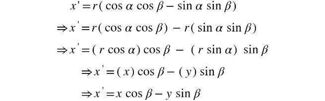
Figure 2.9: Simplified equation for x'
Similarly, let's simplify the equation for y' using the following trigonometric identity:
sin(α + β) = sin α cos β – cos α sin β
Using the preceding equation, we can simplify y' as follows:
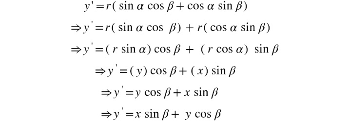
Figure 2.10: Simplified equation for y'
We can now represent x' and y' using the following matrix equation:

Figure 2.11: Representing x' and y' using the matrix equation
Now that we have obtained the preceding equation, we can transform any point into a new point if it's rotated by a given angle. The same equation can be applied to every pixel in an image to obtain the rotated image.
But have you ever seen a rotated image? Even though it's rotated, it still lies within a rectangle. This means the dimensions of the new image can change, unlike in translation, where the dimensions of the output image and the input image stayed the same. Let's see how we can find the dimensions of the image.
Finding the Size of the Output Image
We will consider two cases here. The first case is that we keep the dimensions of the output image the same as the ones for the input image, while the second case is that we modify the dimensions of the output image. Let's understand the difference between them by looking at the following diagram. The left half shows the case when the image dimensions are kept the same, even after rotation, whereas in the right half of the diagram, we relax the dimensions to cover the entire rotated image. You can see the difference in the results obtained in both cases. In the following diagram, L and H refer to the dimensions of the original image, while L' and H' refer to the dimensions after rotation.
The image is rotated by an angle, ϴ, in an anti-clockwise direction, around the center of the image:
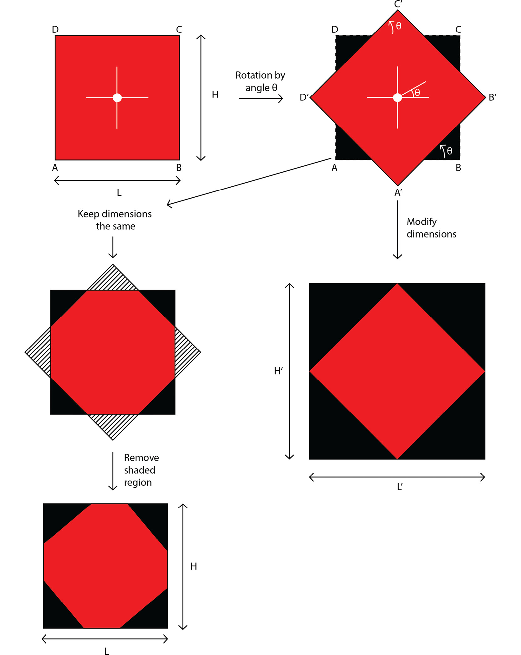
Figure 2.12: Size of the rotated image
In Figure 2.12, the size of the rotated image is presented depending on whether the image dimensions are kept the same or are modified while rotating the image
For the case where we want to keep the size of the image the same as the initial image's size, we just crop out the extra region. Let's learn how to obtain the size of the rotated image, if we don't want to keep the dimensions the same:
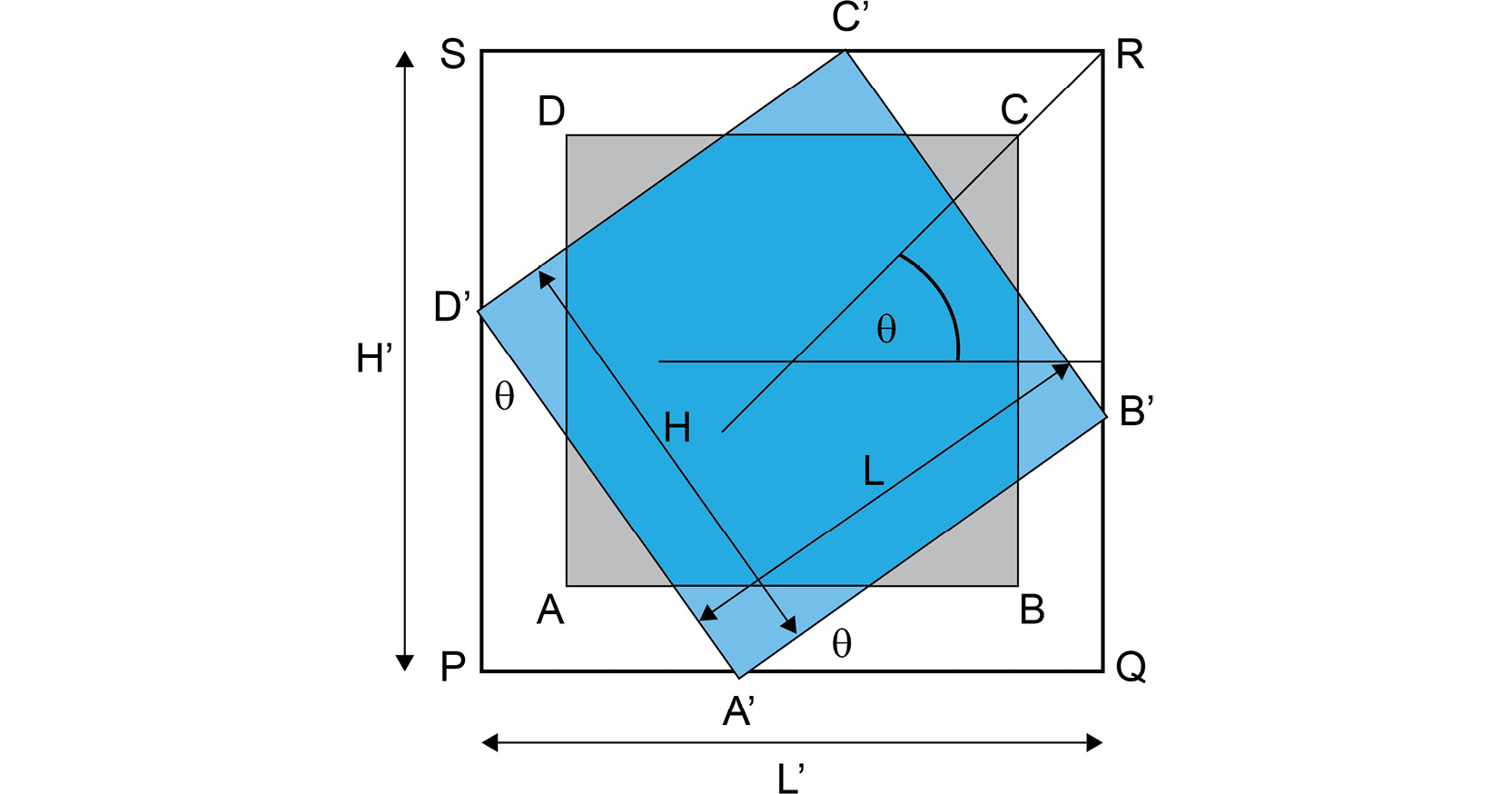
Figure 2.13: Size of the image after rotation
In the preceding diagram, the original image, ABCD, has been rotated along the center of the image by an angle, θ, to form the new image A'B'C'D'.
Referring to the preceding diagram, we can write the following equations:
A'Q = L cos θ
A›P = H sin θ
Thus, we can obtain L' in terms of L and H as follows. Note that L' refers to the size of the image after rotation. Refer to the preceding diagram for a visual representation:
L' = PQ = PA' + A'Q = H sin θ + L cos θ
Similarly, we can write the following equations:
PD' = H cos θ
D›S = L sin θ
Thus, we can obtain H' in terms of L and H, as follows:
H' = PS = PD' + D'S = L sin θ + H cos θ
Here comes a tricky part. We know the values of cosine and sine can also be negative, but the size of the rotated image cannot be smaller than the size of the input image. Thus, we will use the absolute values of sine and cosine. The equations for L' and H' will be modified so that they look as follows:
L' = L|cos θ| + H | sin θ|
H› = L|sin θ| + H | cos θ|
We can round off these values to obtain an integer value for the new width and height of the rotated image.
Now comes the question that you might be wanting to ask by now. Do we have to do all this calculation every time we want to rotate an image? Luckily, the answer is no. OpenCV has a function that we can use if we want to rotate an image by a given angle. It also gives you the option of scaling the image. The function we are talking about here is the cv2.getRotationMatrix2D function. It generates the rotation matrix that can be used to rotate the image. This function takes three arguments:
- The point that we want to rotate the image around. Usually, the center of the image or the bottom-left corner is chosen as the point.
- The angle in degrees that we want to rotate the image by.
- The factor that we want to change the dimensions of the image by. This is an optional argument and can be used to shrink or enlarge the image. In the preceding case, it was 1 as we didn't resize the image.
Note that we are only generating the rotation matrix here and not actually carrying out the rotation. We will cover how to use this matrix when we will look at affine transformations. For now, let's have a look at image resizing.
Image Resizing
Imagine that you are training a deep learning model or using it to carry out some prediction – for example, object detection, image classification, and so on. Most deep learning models (that are used for images) require the input image to be of a fixed size. In such situations, we resize the image to match those dimensions. Image resizing is a very simple concept where we modify an image's dimensions. This concept has its applications in almost every computer vision domain (image classification, face detection, face recognition, and so on).
Images can be resized in two ways:
- Let's say that we have the initial dimensions as
W×H, whereWandHstand for width and height, respectively. If we want to double the size (dimensions) of the image, we can resize or scale the image up to2W×2H. Similarly, if we want to reduce the size (dimensions) of the image by half, then we can resize or scale the image down toW/2×H/2. Since we just want to scale the image, we can pass the scaling factors (for length and width) while resizing. The output dimensions can be calculated based on these scaling factors. - We might want to resize an image to a fixed dimension, let's say,
420×360pixels. In such a situation, scaling won't work as you can't be sure that the initial dimensions are going to be a multiple (or factor) of the fixed dimension. This requires us to pass the new dimensions of the image directly while resizing.
A very interesting thing happens when we resize an image. Let's try to understand this with the help of an example:

Figure 2.14: Image to resize
The preceding figure shows the image and the pixel values that we want to resize. Currently, it's of size 5×5. Let's say we want to double the size. This results in the following output. However, we want to fill in the pixel values:
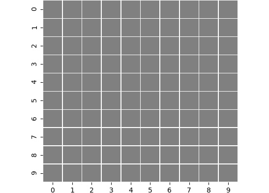
Figure 2.15: Resized image
Let's look at the various options we have. We can always replicate the pixels. This will give us the result shown in the following figure:

Figure 2.16: Resized image by replicating pixel values
If we remove the pixel values from the preceding image, we will obtain the image shown in the following figure. Compare this with the original image, Figure 2.14. Notice how similar it looks to the original image:
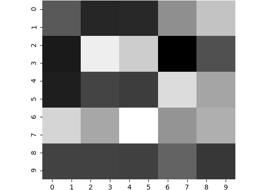
Figure 2.17: Resized image without annotation
Similarly, if we want to reduce the size of the image by half, we can drop some pixels. One thing that you would have noticed is that while resizing, we are replicating the pixels, as shown in Figure 2.16 and Figure 2.17. There are some other techniques we can use as well. We can use interpolation, in which we find out the new pixel values based on the pixel values of the neighboring pixels, instead of directly replicating them. This gives a nice smooth transition in colors. The following figure shows how the results vary if we use different interpolations. From the following figure, we can see that as we progress from left to right, the pixel values of the newly created pixels are calculated differently. In the first three images, the pixels are directly copied from the neighboring pixels, whereas in the later images, the pixel values depend on all the neighboring pixels (left, right, up, and down) and, in some cases, the diagonally adjacent pixels as well:
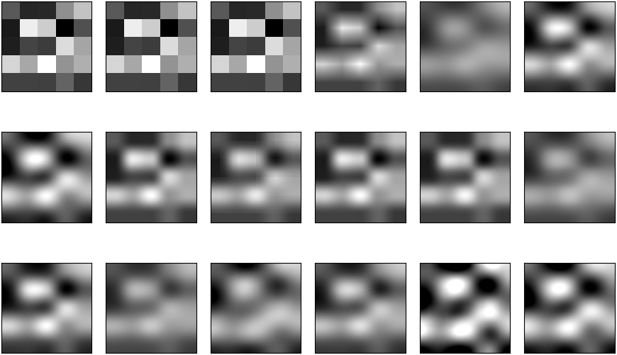
Figure 2.18: Different results obtained based on different interpolations used
Now, you don't need to worry about all the interpolations that are available. We will stick to the following three interpolations for resizing:
- If we are shrinking an image, we will use bilinear interpolation. This is represented as
cv2.INTER_AREAin OpenCV. - If we are increasing the size of an image, we will use either linear interpolation (
cv2.INTER_LINEAR) or cubic interpolation (cv2.INTER_CUBIC).
Let's look at how we can resize an image using OpenCV's cv2.resize function:
cv2.resize(src, dsize, fx, fy, interpolation)
Let's have a look at the arguments of this function:
src: This argument is the image we want to resize.dsize: This argument is the size of the output image (width, height). This will be used when you know the size of the output image. If we are just scaling the image, we will set this toNone.fxandfy: These arguments are the scaling factors. These will only be used when we want to scale the image. If we already know the size of the output image, we will skip these arguments. These arguments are specified asfx = 5, fy = 3, if we want to scale the image by five in thexdirection and three in theydirection.interpolation: This argument is the interpolation that we want to use. This is specified asinterpolation = cv2.INTER_LINEARif we want to use linear interpolation. The other interpolation flags have already been mentioned previously –cv2.INTER_AREAandcv2.INTER_CUBIC.
Next, let's have a look at a more general transformation – affine transformation.
Affine Transformation
Affine transformation is one of the most important geometric transformations in computer vision. The reason for this is that an affine transformation can combine the effects of translation, rotation, and resizing into one transform. Affine transformation in OpenCV uses a 2×3 matrix and then applies the effect using the matrix using the cv2.warpAffine function. This function takes three arguments:
cv2.warpAffine(src, M, dsize)
Let's take a look at each argument:
- The first argument (
src) is the image that we want to apply the transformation to. - The second argument (
M) is the transformation matrix. - The third argument (
dsize) is the shape of the output image. The order that's used is (width, height) or (number of columns, number of rows).
Let's have a look at the transformation matrices for different transformations and how to generate them:
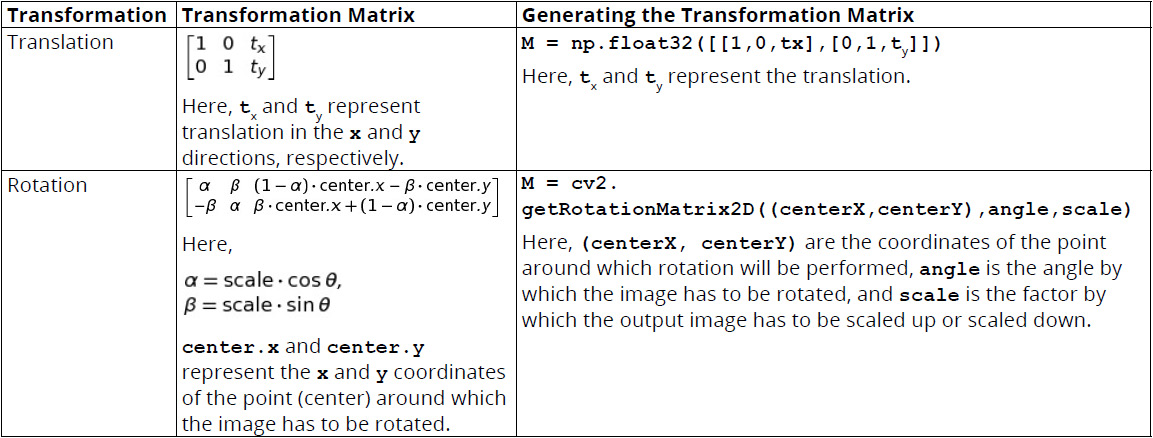
Figure 2.19: Table with transformation matrices for different transformations
To generate the transformation matrix for affine transformation, we choose any three non-collinear points on the input image and the corresponding points on the output image. Let's call the points (in1x, in1y), (in2x, in2y), (in3x, in3y) for the input image, and (out1x, out1y), (out2x, out2y), (out3x, out3y) for the output image.
Then, we can use the following code to generate the transformation matrix. We can use the following code to create a NumPy array for storing the points:
ptsInput = np.float32([[in1x, in1y],[in2x, in2y],\
                      [in3x, in3y]])
Alternatively, we can also use the following code:
ptsOutput = np.float32([[out1x, out1y], [out2x, out2y], \
                       [out3x, out3y]])
Next, we will pass these two NumPy arrays to the cv2.getAffineTransform function, as follows:
M = cv2.getAffineTransform(ptsInput, ptsOutput)
Now that we have seen how to generate the transformation matrix, let's see how to apply it. This can be done using outputImage = cv2.warpAffine(inputImage, M, (outputImageWidth, outputImageHeight)).
Now that we have discussed affine transformation and how to apply it, let's put this knowledge to use in the following exercise.
Exercise 2.02: Working with Affine Transformation
In this exercise, we will use the OpenCV functions that we discussed in the previous sections to translate, rotate, and resize an image. We will be using the following image in this exercise.
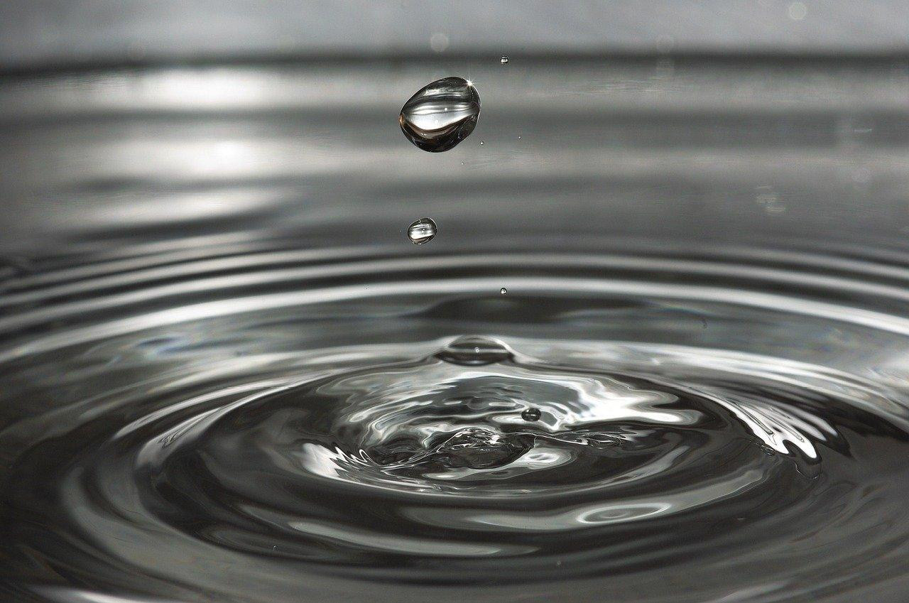
Figure 2.20: Image of a drop
Note
This image is available at https://packt.live/3geu9Hh.
Follow these steps to complete this exercise:
- Create a new Jupyter Notebook –
Exercise2.02.ipynb. We will be writing our code in this notebook. - Start by importing the required modules:
# Import modules
import cv2
import numpy as np
import matplotlib.pyplot as plt
%matplotlib inline
- Next, read the image.
Note
Before proceeding, be sure to change the path to the image (highlighted) based on where the image is saved in your system.
The code is as follows:
img = cv2.imread("../data/drip.jpg") - Display the image using Matplotlib:
plt.imshow(img[:,:,::-1])
plt.show()
The output is as follows. The X and Y axes refer to the width and height of the image, respectively:

Figure 2.21: Image with X and Y axes
- Convert the image into grayscale for ease of use:
img = cv2.cvtColor(img, cv2.COLOR_BGR2GRAY)
- Store the height and width of the image:
height,width = img.shape
- Start with translation. Shift the image by 100 pixels to the right and 100 pixels down:
# Translation
tx = 100
ty = 100
M = np.float32([[1,0,tx],[0,1,ty]])
dst = cv2.warpAffine(img,M,(width,height))
plt.imshow(dst,cmap="gray")
plt.show()
The preceding code produces the following output. The X and Y axes refer to the width and height of the image, respectively:

Figure 2.22: Translated image
- Next, rotate our image 45 degrees anti-clockwise, around the center of the image, and scale it up twice:
# Rotation
angle = 45
center = (width//2, height//2)
scale = 2
M = cv2.getRotationMatrix2D(center,angle,scale)
dst = cv2.warpAffine(img,M,(width,height))
plt.imshow(dst,cmap="gray")
plt.show()
The output is as follows. The X and Y axes refer to the width and height of the image, respectively:

Figure 2.23: Rotated image
- Finally, double the size of the image using the
cv2.resizefunction:# Resizing image print("Width of image = {}, Height of image = {}"\ .format(width, height)) dst = cv2.resize(img, None, fx=2, fy=2, \ interpolation=cv2.INTER_LINEAR) height, width = dst.shape print("Width of image = {}, Height of image = {}"\ .format(width, height))The output is as follows:
Width of image = 1280, Height of image = 849
Width of image = 2560, Height of image = 1698
In this exercise, we learned how to translate, rotate, and resize an image using OpenCV functions.
Note
To access the source code for this specific section, please refer to https://packt.live/38iUnFZ.
Next, let's have a look at the final geometric transformation of this chapter – perspective transformation.
Perspective Transformation
Perspective transformation, unlike all the transformations we have seen so far, requires a 3×3 transformation matrix. We won't go into the mathematics behind this matrix as it's out of the scope of this book. We will need four points in the input image and the coordinates of the same points in the output image. Note that these points should not be collinear. Next, similar to the affine transformation steps, we will carry out perspective transformation.
We will use the following code create a NumPy array for storing the points:
ptsInput = np.float32([[in1x, in1y],[in2x, in2y],[in3x, in3y],\
                      [in4x,in4y]])
Alternatively, we can use the following code:
ptsOutput = np.float32([[out1x, out1y], [out2x, out2y], \
                       [out3x, out3y], [out4x, out4y]])
Next, we will pass these two NumPy arrays to the cv2.getPerspectiveTransform function:
M = cv2.getPerspectiveTransform(ptsInput, ptsOutput)
The transformation matrix can then be applied using the following code:
outputImage = cv2.warpPerspective(inputImage, M, \
              (outputImageWidth, outputImageHeight))
The primary difference between perspective and affine transformation is that in perspective transformation, straight lines will still remain straight after the transformation, unlike in affine transformation, where, because of multiple transformations, the line can be converted into a curve.
Let's see how we can use perspective transformation with the help of an exercise.
Exercise 2.03: Perspective Transformation
In this exercise, we will carry out perspective transformation to obtain the front cover of the book given as the input image. We will use OpenCV's cv2.getPerspectiveTransform and cv2.warpPerspective functions. We will be using the following image of a book:

Figure 2.24: Image of a book
Note
This image can be downloaded from https://packt.live/2YM9tAA.
Follow these steps to complete this exercise:
- Create a new Jupyter Notebook –
Exercise2.03.ipynb. We will be writing our code in this notebook. - Import the modules we will be using:
# Import modules
import cv2
import numpy as np
import matplotlib.pyplot as plt
%matplotlib inline
- Next, read the image.
Note
Before proceeding, be sure to change the path to the image (highlighted) based on where the image is saved in your system.
The code is as follows:
img = cv2.imread("../data/book.jpg") - Display the image using Matplotlib, as follows:
plt.imshow(img[:,:,::-1])
plt.show()
The output is as follows. The X and Y axes refer to the width and height of the image, respectively:

Figure 2.25: Output image of a book
- Specify four points in the image so that they lie at the four corners of the front cover. Since we just want the front cover, the output points will be nothing but the corner points of the final 300×300 image. Note that the order of the points should stay the same for both the input and output points:
inputPts = np.float32([[4,381],
                      [266,429],
                      [329,68],
                      [68,20]])
outputPts = np.float32([[0,300],
                       [300,300],
                       [300,0],
                       [0,0]])
- Next, obtain the transformation matrix:
M = cv2.getPerspectiveTransform(inputPts,outputPts)
- Apply this transformation matrix to carry out perspective transformation:
dst = cv2.warpPerspective(img,M,(300,300))
- Display the resultant image using Matplotlib. The X and Y axes refer to the width and height of the image, respectively:
plt.imshow(dst[:,:,::-1])
plt.show()

Figure 2.26: Front cover of the book
In this exercise, we saw how we can use geometric transformations to extract the front cover of the book provided in a given image. This can be interesting when we are trying to scan a document and we want to obtain a properly oriented image of the document after scanning.
Note
To access the source code for this specific section, please refer to https://packt.live/2YOqs5u.
With that, we have covered all the major geometric transformations. It's time to cover another important topic in image processing – image arithmetic.