Binary Images
So far, we have worked with images with one channel (grayscale images) and three channels (color images). We also mentioned that, usually, pixel values in images are represented as 8-bit unsigned integers and that's why they have a range from 0 to 255. But that's not always true. Images can be represented using floating-point values and also with lesser bits, which also reduces the range. For example, an image using 6-bit unsigned integers will have a range between 0 - (26-1) or 0 to 63.
Even though it's possible to use more or fewer bits, typically, we work with only two kinds of ranges – 0 to 255 for 8-bit unsigned integers and images that have only 0 and 1. The second category of images uses only two pixel values, and that's why they are referred to as binary images. Binary images need only a single bit to represent a pixel value. These images are commonly used as masks for selecting or removing a certain region of an image. It is with these images that bitwise operations are commonly used. Can you think of a place where you have seen binary images in real life?
You can find such black-and-white images quite commonly in QR codes. Can you think of some other applications of binary images? Binary images are extensively used for document analysis and even in industrial machine vision tasks. Here is a sample binary image:

Figure 2.37: QR code as an example of a binary image
Now, let's see how we can convert an image into a binary image. This technique comes under the category of thresholding. Thresholding refers to the process of converting a color image into a binary image. There is a wide range of thresholding techniques available, but here, we will focus only on a very simple thresholding technique – binary thresholding – since we are working with binary images.
The concept behind binary thresholding is very simple. You choose a threshold value and all the pixel values below and equal to the threshold are replaced with 0, while all the pixel values above the threshold are replaced with a specified value (usually 1 or 255). This way, you end up with an image that has only two unique pixel values, which is what a binary image is.
We can convert an image into a binary image using the following code:
# Set threshold and maximum value
thresh = 125
maxValue = 255
# Binary threshold
th, dst = cv2.threshold(img, thresh, maxValue, \
                        cv2.THRESH_BINARY)
In the preceding code, we first specified the threshold as 125 and then specified the maximum value. This is the value that will replace all the pixel values above the threshold. Finally, we used OpenCV's cv2.threshold function to perform binary thresholding. This function takes the following inputs:
- The grayscale image that we want to perform thresholding on.
thresh: The threshold value.maxValue: The maximum value, which will replace all pixel values above the threshold.th,dst: The thresholding flag. Since we are performing binary thresholding, we will usecv2.THRESH_BINARY.
Let's implement what we've learned about binary thresholding.
Exercise 2.06: Converting an Image into a Binary Image
In this exercise, we will use binary thresholding to convert a color image into a binary image. We will be working on the following image of zebras:
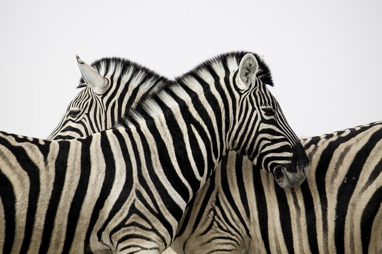
Figure 2.38: Image of zebras
Note
This image can be found at https://packt.live/2ZpQ07Z .
Follow these steps to complete this exercise:
- Create a new Jupyter Notebook –
Exercise2.06.ipynb. We will be writing our code in this notebook. - Import the necessary modules:
# Import modules
import cv2
import numpy as np
import matplotlib.pyplot as plt
%matplotlib inline
- Read the image of the zebras and convert it into grayscale. This is necessary because we know that thresholding requires us to provide a grayscale image as an argument.
Note
Before proceeding, be sure to change the path to the image (highlighted) based on where the image is saved in your system.
The code for this is as follows:
img = cv2.imread("../data/zebra.jpg") img = cv2.cvtColor(img, cv2.COLOR_BGR2GRAY) - Display the grayscale image using Matplotlib:
plt.imshow(img, cmap='gray')
plt.show()
The output is as follows. The X and Y axes refer to the width and height of the image, respectively:

Figure 2.39: Image in grayscale
- Use the
cv2.thresholdingfunction and set the threshold to150:# Set threshold and maximum value thresh = 150 maxValue = 255 # Binary threshold th, dst = cv2.threshold(img, thresh, maxValue, \ cv2.THRESH_BINARY)
Note
You can try playing around with the threshold value to obtain different results.
- Display the binary image we have obtained:
plt.imshow(dst, cmap='gray')
plt.show()
The output is as follows. The X and Y axes refer to the width and height of the image, respectively:

Figure 2.40: Binary image
Note
To access the source code for this specific section, please refer to https://packt.live/2VyYHfa.
In this exercise, we saw how to obtain a binary image using thresholding. Next, let's see how we can carry out bitwise operations on these images.
Bitwise Operations on Images
Let's start by listing the binary operations, along with their results. You must have read about these operations before, so we won't go into their details. The following table provides the truth tables for the bitwise operations as a quick refresher:
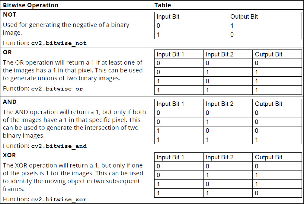
Figure 2.41: Bitwise operations and truth tables
Let's see how we can use these functions with the help of an exercise.
Exercise 2.07: Chess Pieces
In this exercise, we will use the XOR operation to find the chess pieces that have moved using two images taken of the same chess game:
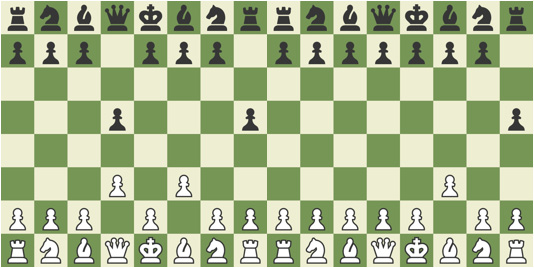
Figure 2.42: Two images of chess board
Note
These images can be found at https://packt.live/3fuxLoU.
Follow these steps to complete this exercise:
- Create a new notebook –
Exercise2.07.ipynb. We will be writing our code in this notebook. - Import the required modules:
# Import modules
import cv2
import numpy as np
import matplotlib.pyplot as plt
%matplotlib inline
- Read the images of the board and convert them to grayscale.
Note
Before proceeding, be sure to change the path to the images (highlighted) based on where the images are saved in your system.
The code for this is as follows:
img1 = cv2.imread("../data/board.png") img2 = cv2.imread("../data/board2.png") img1 = cv2.cvtColor(img1, cv2.COLOR_BGR2GRAY) img2 = cv2.cvtColor(img2, cv2.COLOR_BGR2GRAY) - Display these images using Matplotlib:
plt.imshow(img1,cmap="gray")
plt.show()
The output is as follows. The X and Y axes refer to the width and height of the image, respectively:

Figure 2.43: Grayscale version of the chess image
- Plot the second image, as follows:
plt.imshow(img2,cmap="gray")
plt.show()
The output is as follows. The X and Y axes refer to the width and height of the image, respectively:

Figure 2.44: Grayscale version of the chess image
- Threshold both the images using a threshold value of 150 and a maximum value of 255:
# Set threshold and maximum value
thresh = 150
maxValue = 255
# Binary threshold
th, dst1 = cv2.threshold(img1, thresh, maxValue, \
                         cv2.THRESH_BINARY)
# Binary threshold
th, dst2 = cv2.threshold(img2, thresh, maxValue, \
                         cv2.THRESH_BINARY)
- Display these binary images using Matplotlib:
plt.imshow(dst1, cmap='gray')
plt.show()
The output is as follows. The X and Y axes refer to the width and height of the image, respectively:

Figure 2.45: Binary image
- Print the second image, as follows:
plt.imshow(dst2, cmap='gray')
plt.show()
The output is as follows. The X and Y axes refer to the width and height of the image, respectively:

Figure 2.46: Image after thresholding
- Use bitwise XOR to find the pieces that have moved, as follows:
dst = cv2.bitwise_xor(dst1,dst2)
- Display the result, as follows. The X and Y axes refer to the width and height of the image, respectively:
plt.imshow(dst, cmap='gray')
plt.show()
The output is as follows:

Figure 2.47: Result of the XOR operation
Notice that, in the preceding image, the four pieces that are present show the initial and final positions of the only two pieces that had changed their positions in the two images. In this exercise, we used the XOR operation to perform motion detection to detect the two chess pieces that had moved their positions after a few steps.
Note
To access the source code for this specific section, please refer to https://packt.live/2NHixQY.
Masking
Let's discuss one last concept related to binary images. Binary images are quite frequently used to serve as a mask. For example, consider the following image. We will be using an image of a disk:
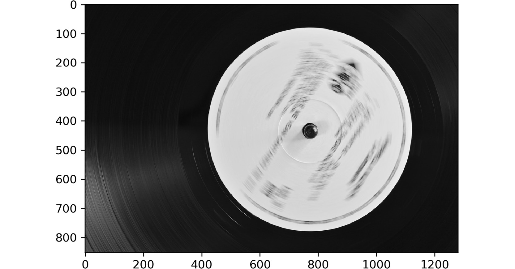
Figure 2.48: Image of a disk
After image thresholding, the mask will look as follows:
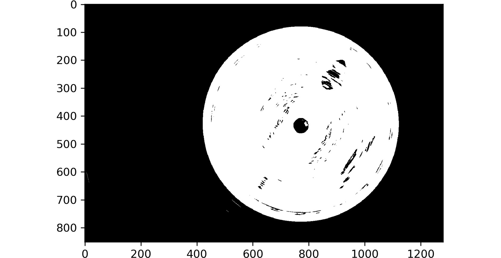
Figure 2.49: Binary mask
Let's see what happens when we apply masking to the image of the zebras that we worked with earlier:
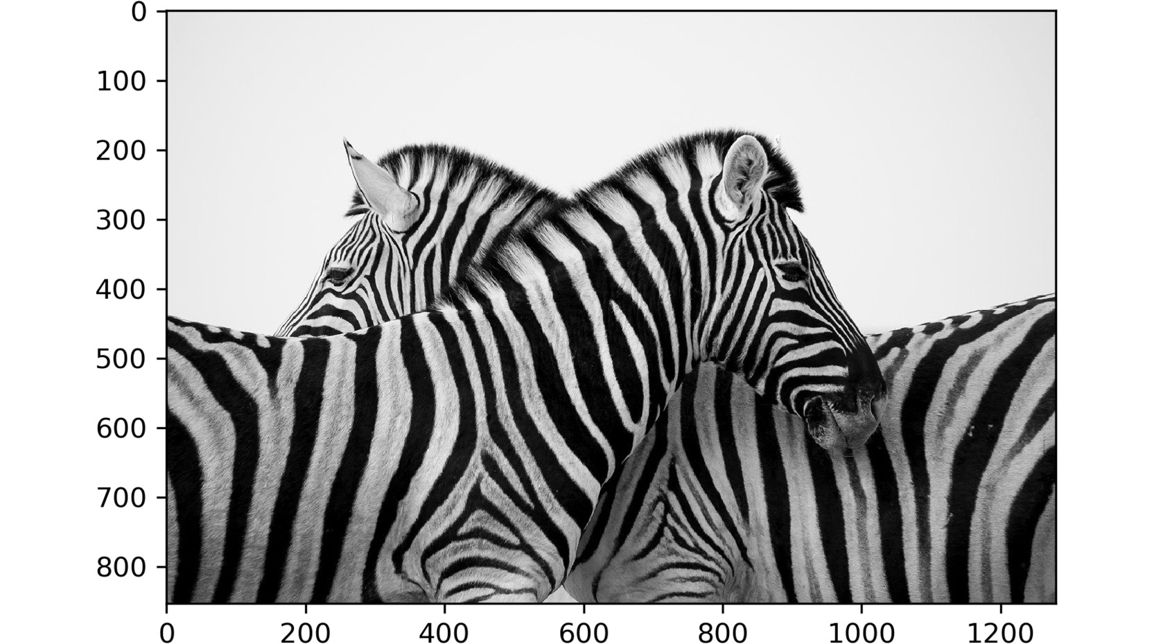
Figure 2.50: Image of zebras
The final image will look as follows:

Figure 2.51: Final image
Let's start with Figure 2.49. This image is a binary image of a disk after thresholding. Figure 2.50 shows the familiar grayscale image of zebras. When Figure 2.49 is used as a mask to only keep the pixels of Figure 2.50, where the corresponding pixels of Figure 2.50 are white, we end up with the result shown in Figure 2.51. Let's break this down. Consider a pixel, P, at location (x,y) in Figure 2.49. If the pixel, P, is white or non-zero (because zero refers to black), the pixel at location (x,y) in Figure 2.50 will be left as it is. If the pixel, P, was black or zero, the pixel at location (x,y) in Figure 2.50 will be replaced with 0. This refers to a masking operation since Figure 2.49 is covering Figure 2.50 as a mask and displaying only a few selected pixels. Such an operation can be easily carried out using the following code:
result = np.where(mask, image, 0)
Let's understand what is happening here. NumPy's np.where function says that wherever the mask (first argument) is non-zero, return the value of the image (second argument); otherwise, return 0 (third argument). This is exactly what we discussed in the previous paragraph. We will be using masks in Chapter 5, Face Processing in Image and Video, as well.
Now, it's time for you to try out the concepts that you have studied so far to replicate the result shown in Figure 2.51.
Activity 2.01: Masking Using Binary Images
In this activity, you will be using masking and other concepts you've studied in this chapter to replicate the result shown in Figure 2.51. We will be using image resizing, image thresholding, and image masking concepts to display only the heads of the zebras present in Figure 2.50. A similar concept can be applied to create nice portraits of photos where only the face of the person is visible and the rest of the region/background is blacked out. Let's start with the steps that you need to follow to complete this activity:
- Create a new notebook –
Activity2.01.ipynb. You will be writing your code in this notebook. - Import the necessary libraries – OpenCV, NumPy, and Matplotlib. You will also need to add the magic command to display images inside the notebook.
- Read the image titled
recording.jpgfrom the disk and convert it to grayscale.Note
This image can be found at https://packt.live/32c3pDK.
- Next, you will have to perform thresholding on this image. You can use a threshold of 150 and a maximum value of 255.
- The thresholded image should be similar to the one shown in Figure 2.49.
- Next, read the image of the zebras (titled
zebras.jpg) and convert it to grayscale.Note
This image can be found at https://packt.live/2ZpQ07Z.
- Before moving on to using NumPy's
wherecommand for masking, we need to check whether the images have the same size or not. Print the shapes of both images (zebras and disk). - You will notice that the images have different dimensions. Resize both images to 1,280×800 pixels. This means that the width of the resized image should be 1,280 pixels and that the height should be 800 pixels. You will have to use the
cv2.resizefunction for resizing. Use linear interpolation while resizing the images. - Next, use NumPy's
wherecommand to only keep the pixels where the disk pixels are white. The other pixels should be replaced with black color.
By completing this activity, you will get an output similar to the following:
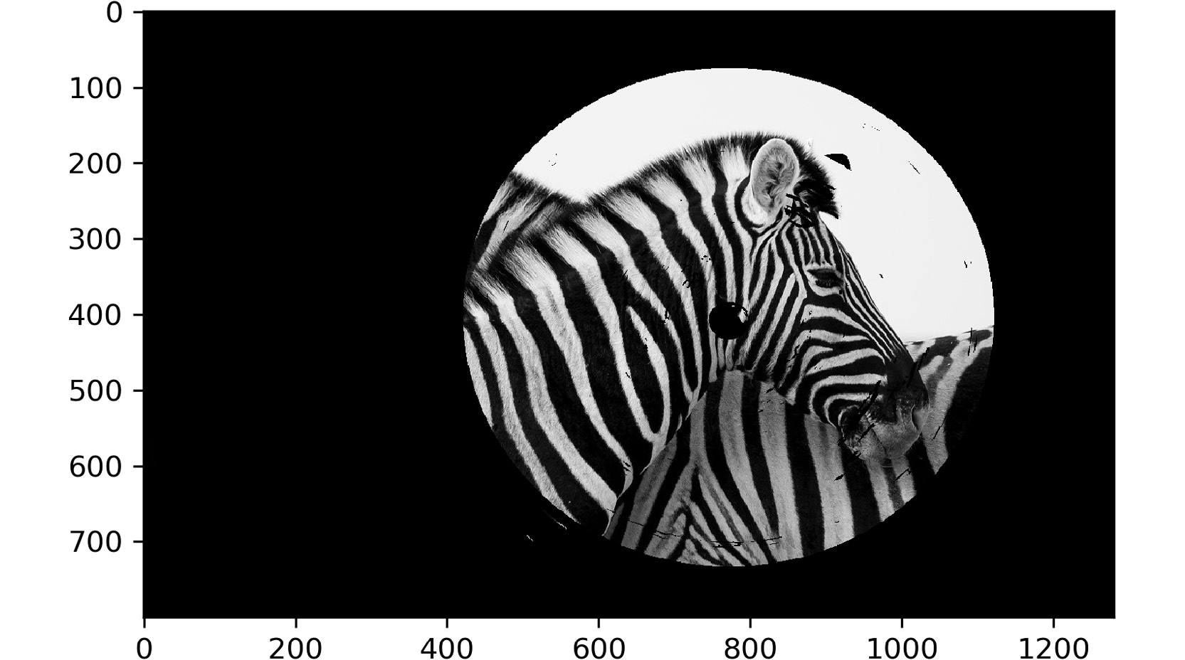
Figure 2.52: Zebra image
The result that we have obtained in this activity can be used in portrait photography, where only the subject of the image is highlighted and the background is replaced with black.
Note
The solution for this activity can be found via this link.
By completing this activity, you have learned how to use image resizing to change the shape of an image, image thresholding to convert a color image into a binary image, and bitwise operations to perform image masking. Notice how image masking can be used to "mask" or hide certain regions of an image and display only the remaining portion of the image. This technique is used extensively in document analysis in computer vision.