Digging into the core of machine learning
After discussing the categorization of machine learning algorithms, we are going to dig into the core of machine learning—generalizing with data, and different levels of generalization, as well as the approaches to attain the right level of generalization.
Generalizing with data
The good thing about data is that there's a lot of it in the world. The bad thing is that it's hard to process this data. The challenge stems from the diversity and noisiness of the data. We humans usually process data coming into our ears and eyes. These inputs are transformed into electrical or chemical signals. On a very basic level, computers and robots also work with electrical signals. These electrical signals are then translated into ones and zeros. However, we program in Python in this book and, on that level, normally we represent the data either as numbers, images, or texts. Actually, images and text aren't very convenient, so we need to transform images and text into numerical values.
Especially in the context of supervised learning, we have a scenario similar to studying for an exam. We have a set of practice questions and the actual exams. We should be able to answer exam questions without knowing the answers to them. This is called generalization—we learn something from our practice questions and, hopefully, are able to apply the knowledge to other similar questions. In machine learning, these practice questions are called training sets or training samples. This is where the machine learning models derive patterns from. And the actual exams are testing sets or testing samples. They are where the models eventually apply to. And learning effectiveness is measured by the compatibility of the learning models and the testing. Sometimes, between practice questions and actual exams, we have mock exams to assess how well we will do in actual exams and to aid revision. These mock exams are known as validation sets or validation samples in machine learning. They help us to verify how well the models will perform in a simulated setting, and then we fine-tune the models accordingly in order to achieve greater hits.
An old-fashioned programmer would talk to a business analyst or other expert, and then implement a tax rule that adds a certain value multiplied by another corresponding value, for instance. In a machine learning setting, we can give the computer a bunch of input and output examples; or, if we want to be more ambitious, we can feed the program the actual tax texts. We can let the machine consume the data and figure out the tax rule, just as an autonomous car doesn't need a lot of explicit human input.
In physics, we have almost the same situation. We want to know how the universe works and formulate laws in a mathematical language. Since we don't know the actual function, all we can do is measure the error produced and try to minimize it. In supervised learning tasks, we compare our results against the expected values. In unsupervised learning, we measure our success with related metrics. For instance, we want clusters of data to be well defined; the metrics could be how similar the data points within one cluster are, and how different the data points from two clusters are. In reinforcement learning, a program evaluates its moves, for example, using a predefined function in a chess game.
Aside from correct generalization with data, there can be two levels of generalization, overfitting and underfitting, which we will explore in the next section.
Overfitting, underfitting, and the bias-variance trade-off
Let's take a look at both levels in detail and also explore the bias-variance trade-off.
Overfitting
Reaching the right fit model is the goal of a machine learning task. What if the model overfits? Overfitting means a model fits the existing observations too well but fails to predict future new observations. Let's look at the following analogy.
If we go through many practice questions for an exam, we may start to find ways to answer questions that have nothing to do with the subject material. For instance, given only five practice questions, we might find that if there are two occurrences of potatoes, one of tomato, and three of banana in a question, the answer is always A, and if there is one occurrence of potato, three of tomato, and two of banana in a question, the answer is always B. We could then conclude that this is always true and apply such a theory later on, even though the subject or answer may not be relevant to potatoes, tomatoes, or bananas. Or, even worse, we might memorize the answers to each question verbatim. We would then score highly on the practice questions, leading us to hope that the questions in the actual exams would be the same as the practice questions. However, in reality, we would score very low on the exam questions as it's rare that the exact same questions occur in exams.
The phenomenon of memorization can cause overfitting. This can occur when we're over extracting too much information from the training sets and making our model just work well with them, which is called low bias in machine learning. In case you need a quick recap of bias, here it is: bias is the difference between the average prediction and the true value. It is computed as follows:

Here, ŷ is the prediction. At the same time, however, overfitting won't help us to generalize to new data and derive true patterns from it. The model, as a result, will perform poorly on datasets that weren't seen before. We call this situation high variance in machine learning. Again, a quick recap of variance: variance measures the spread of the prediction, which is the variability of the prediction. It can be calculated as follows:

The following example demonstrates what a typical instance of overfitting looks like, where the regression curve tries to flawlessly accommodate all observed samples:
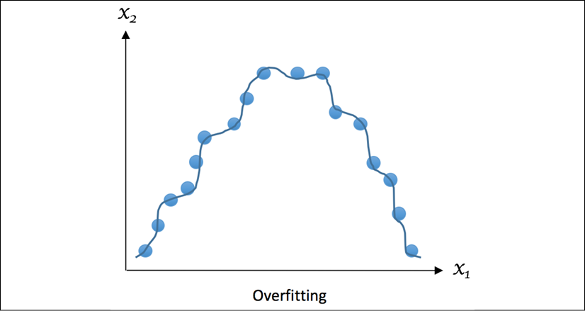
Figure 1.6: Example of overfitting
Overfitting occurs when we try to describe the learning rules based on too many parameters relative to the small number of observations, instead of the underlying relationship, such as the preceding example of potato and tomato, where we deduced three parameters from only five learning samples. Overfitting also takes place when we make the model excessively complex so that it fits every training sample, such as memorizing the answers for all questions, as mentioned previously.
Underfitting
The opposite scenario is underfitting. When a model is underfit, it doesn't perform well on the training sets and won't do so on the testing sets, which means it fails to capture the underlying trend of the data. Underfitting may occur if we aren't using enough data to train the model, just like we will fail the exam if we don't review enough material; this may also happen if we're trying to fit a wrong model to the data, just like we will score low in any exercises or exams if we take the wrong approach and learn it the wrong way. We call any of these situations a high bias in machine learning; although its variance is low as the performance in training and test sets is pretty consistent, in a bad way.
The following example shows what a typical underfitting looks like, where the regression curve doesn't fit the data well enough or capture enough of the underlying pattern of the data:
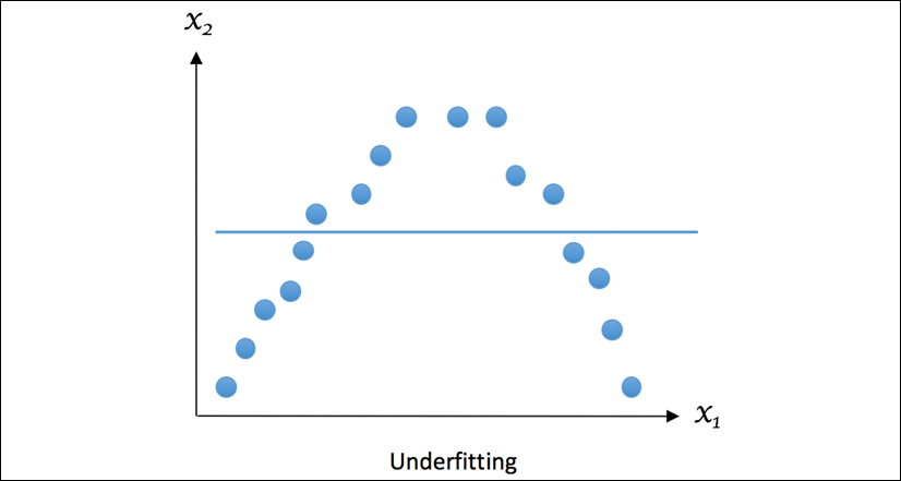
Figure 1.7: Example of underfitting
Now, let's look at what a well-fitting example should look like:
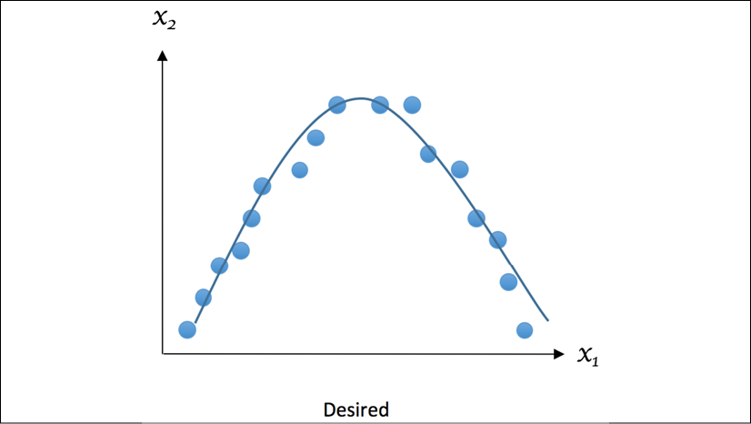
Figure 1.8: Example of desired fitting
The bias-variance trade-off
Obviously, we want to avoid both overfitting and underfitting. Recall that bias is the error stemming from incorrect assumptions in the learning algorithm; high bias results in underfitting. Variance measures how sensitive the model prediction is to variations in the datasets. Hence, we need to avoid cases where either bias or variance is getting high. So, does it mean we should always make both bias and variance as low as possible? The answer is yes, if we can. But, in practice, there is an explicit trade-off between them, where decreasing one increases the other. This is the so-called bias-variance trade-off. Sounds abstract? Let's take a look at the next example.
Let's say we're asked to build a model to predict the probability of a candidate being the next president in America based on phone poll data. The poll is conducted using zip codes. We randomly choose samples from one zip code and we estimate there's a 61% chance the candidate will win. However, it turns out he loses the election. Where did our model go wrong? The first thing we think of is the small size of samples from only one zip code. It's a source of high bias also, because people in a geographic area tend to share similar demographics, although it results in a low variance of estimates. So, can we fix it simply by using samples from a large number of zip codes? Yes, but don't get happy so early. This might cause an increased variance of estimates at the same time. We need to find the optimal sample size—the best number of zip codes to achieve the lowest overall bias and variance.
Minimizing the total error of a model requires a careful balancing of bias and variance. Given a set of training samples, x1, x2, …, xn, and their targets, y1, y2, …, yn, we want to find a regression function ŷ(x) that estimates the true relation y(x) as correctly as possible. We measure the error of estimation, how good (or bad) the regression model is, in mean squared error (MSE):

The E denotes the expectation. This error can be decomposed into bias and variance components following the analytical derivation, as shown in the following formula (although it requires a bit of basic probability theory to understand):
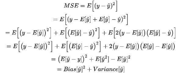
The Bias term measures the error of estimations and the Variance term describes how much the estimation, ŷ, moves around its mean, E[ŷ]. The more complex the learning model ŷ(x) is, and the larger the size of the training samples, the lower the bias will become. However, this will also create more shift to the model in order to better fit the increased data points. As a result, the variance will be lifted.
We usually employ the cross-validation technique as well as regularization and feature reduction to find the optimal model balancing bias and variance and to diminish overfitting. We will talk about these next.
You may ask why we only want to deal with overfitting: how about underfitting? This is because underfitting can be easily recognized: it occurs as long as the model doesn't work well on a training set. And we need to find a better model or tweak some parameters to better fit the data, which is a must under all circumstances. On the other hand, overfitting is hard to spot. Oftentimes, when we achieve a model that performs well on a training set, we are overly happy and think it ready for production right away. This can be very dangerous. We should instead take extra steps to ensure that the great performance isn't due to overfitting and the great performance applies to data excluding the training data.
Avoiding overfitting with cross-validation
As a gentle reminder, you will see cross-validation in action multiple times later in this book. So don't panic if you ever find this section difficult to understand as you will become an expert of it very soon.
Recall that between practice questions and actual exams, there are mock exams where we can assess how well we will perform in actual exams and use that information to conduct necessary revision. In machine learning, the validation procedure helps to evaluate how the models will generalize to independent or unseen datasets in a simulated setting. In a conventional validation setting, the original data is partitioned into three subsets, usually 60% for the training set, 20% for the validation set, and the rest (20%) for the testing set. This setting suffices if we have enough training samples after partitioning and we only need a rough estimate of simulated performance. Otherwise, cross-validation is preferable.
In one round of cross-validation, the original data is divided into two subsets, for training and testing (or validation), respectively. The testing performance is recorded. Similarly, multiple rounds of cross-validation are performed under different partitions. Testing results from all rounds are finally averaged to generate a more reliable estimate of model prediction performance. Cross-validation helps to reduce variability and, therefore, limit overfitting.
When the training size is very large, it's often sufficient to split it into training, validation, and testing (three subsets) and conduct a performance check on the latter two. Cross-validation is less preferable in this case since it's computationally costly to train a model for each single round. But if you can afford it, there's no reason not to use cross-validation. When the size isn't so large, cross-validation is definitely a good choice.
There are mainly two cross-validation schemes in use: exhaustive and non-exhaustive. In the exhaustive scheme, we leave out a fixed number of observations in each round as testing (or validation) samples and use the remaining observations as training samples. This process is repeated until all possible different subsets of samples are used for testing once. For instance, we can apply Leave-One-Out-Cross-Validation (LOOCV), which lets each sample be in the testing set once. For a dataset of the size n, LOOCV requires n rounds of cross-validation. This can be slow when n gets large. This following diagram presents the workflow of LOOCV:
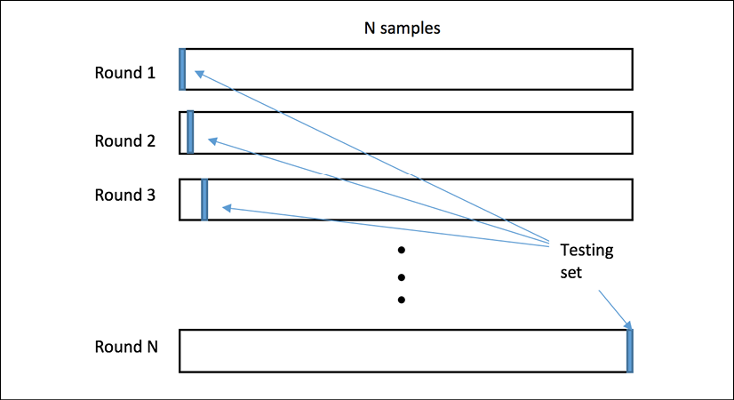
Figure 1.9: Workflow of leave-one-out-cross-validation
A non-exhaustive scheme, on the other hand, as the name implies, doesn't try out all possible partitions. The most widely used type of this scheme is k-fold cross-validation. We first randomly split the original data into k equal-sized folds. In each trial, one of these folds becomes the testing set, and the rest of the data becomes the training set.
We repeat this process k times, with each fold being the designated testing set once. Finally, we average the k sets of test results for the purpose of evaluation. Common values for k are 3, 5, and 10. The following table illustrates the setup for five-fold:
|
Round |
Fold 1 |
Fold 2 |
Fold 3 |
Fold 4 |
Fold 5 |
|
1 |
Testing |
Training |
Training |
Training |
Training |
|
2 |
Training |
Testing |
Training |
Training |
Training |
|
3 |
Training |
Training |
Testing |
Training |
Training |
|
4 |
Training |
Training |
Training |
Testing |
Training |
|
5 |
Training |
Training |
Training |
Training |
Testing |
Table 1.1: Setup for 5-fold cross-validation
K-fold cross-validation often has a lower variance compared to LOOCV, since we're using a chunk of samples instead of a single one for validation.
We can also randomly split the data into training and testing sets numerous times. This is formally called the holdout method. The problem with this algorithm is that some samples may never end up in the testing set, while some may be selected multiple times in the testing set.
Last but not the least, nested cross-validation is a combination of cross-validations. It consists of the following two phases:
- Inner cross-validation: This phase is conducted to find the best fit and can be implemented as a k-fold cross-validation
- Outer cross-validation: This phase is used for performance evaluation and statistical analysis
We will apply cross-validation very intensively throughout this entire book. Before that, let's look at cross-validation with an analogy next, which will help us to better understand it.
A data scientist plans to take his car to work and his goal is to arrive before 9 a.m. every day. He needs to decide the departure time and the route to take. He tries out different combinations of these two parameters on certain Mondays, Tuesdays, and Wednesdays and records the arrival time for each trial. He then figures out the best schedule and applies it every day. However, it doesn't work quite as well as expected.
It turns out the scheduling model is overfit with data points gathered in the first three days and may not work well on Thursdays and Fridays. A better solution would be to test the best combination of parameters derived from Mondays to Wednesdays on Thursdays and Fridays and similarly repeat this process based on different sets of learning days and testing days of the week. This analogized cross-validation ensures that the selected schedule works for the whole week.
In summary, cross-validation derives a more accurate assessment of model performance by combining measures of prediction performance on different subsets of data. This technique not only reduces variance and avoids overfitting, but also gives an insight into how the model will generally perform in practice.
Avoiding overfitting with regularization
Another way of preventing overfitting is regularization. Recall that the unnecessary complexity of the model is a source of overfitting. Regularization adds extra parameters to the error function we're trying to minimize, in order to penalize complex models.
According to the principle of Occam's razor, simpler methods are to be favored. William Occam was a monk and philosopher who, around the year 1320, came up with the idea that the simplest hypothesis that fits data should be preferred. One justification is that we can invent fewer simple models than complex models. For instance, intuitively, we know that there are more high-polynomial models than linear ones. The reason is that a line (y = ax + b) is governed by only two parameters—the intercept, b, and slope, a. The possible coefficients for a line span two-dimensional space. A quadratic polynomial adds an extra coefficient for the quadratic term, and we can span a three-dimensional space with the coefficients. Therefore, it is much easier to find a model that perfectly captures all training data points with a high-order polynomial function, as its search space is much larger than that of a linear function. However, these easily obtained models generalize worse than linear models, which are more prone to overfitting. And, of course, simpler models require less computation time. The following diagram displays how we try to fit a linear function and a high order polynomial function, respectively, to the data:
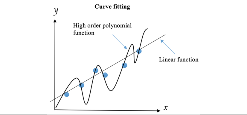
Figure 1.10: Fitting data with a linear function and a polynomial function
The linear model is preferable as it may generalize better to more data points drawn from the underlying distribution. We can use regularization to reduce the influence of the high orders of polynomial by imposing penalties on them. This will discourage complexity, even though a less accurate and less strict rule is learned from the training data.
We will employ regularization quite often starting from Chapter 5, Predicting Online Ad Click-Through with Logistic Regression. For now, let's look at an analogy that can help you better understand regularization.
A data scientist wants to equip his robotic guard dog with the ability to identify strangers and his friends. He feeds it with the following learning samples:
|
Male |
Young |
Tall |
With glasses |
In grey |
Friend |
|
Female |
Middle |
Average |
Without glasses |
In black |
Stranger |
|
Male |
Young |
Short |
With glasses |
In white |
Friend |
|
Male |
Senior |
Short |
Without glasses |
In black |
Stranger |
|
Female |
Young |
Average |
With glasses |
In white |
Friend |
|
Male |
Young |
Short |
Without glasses |
In red |
Friend |
Table 1.2: Training samples for the robotic guard dog
The robot may quickly learn the following rules:
- Any middle-aged female of average height without glasses and dressed in black is a stranger
- Any senior short male without glasses and dressed in black is a stranger
- Anyone else is his friend
Although these perfectly fit the training data, they seem too complicated and unlikely to generalize well to new visitors. In contrast, the data scientist limits the learning aspects. A loose rule that can work well for hundreds of other visitors could be as follows: anyone without glasses dressed in black is a stranger.
Besides penalizing complexity, we can also stop a training procedure early as a form of regularization. If we limit the time a model spends learning or we set some internal stopping criteria, it's more likely to produce a simpler model. The model complexity will be controlled in this way and, hence, overfitting becomes less probable. This approach is called early stopping in machine learning.
Last but not least, it's worth noting that regularization should be kept at a moderate level or, to be more precise, fine-tuned to an optimal level. Too small a regularization doesn't make any impact; too large a regularization will result in underfitting, as it moves the model away from the ground truth. We will explore how to achieve optimal regularization in Chapter 5, Predicting Online Ad Click-Through with Logistic Regression, Chapter 7, Stock Prices Prediction with Regression Algorithms, and Chapter 8, Predicting Stock Prices with Artificial Neural Networks.
Avoiding overfitting with feature selection and dimensionality reduction
We typically represent data as a grid of numbers (a matrix). Each column represents a variable, which we call a feature in machine learning. In supervised learning, one of the variables is actually not a feature, but the label that we're trying to predict. And in supervised learning, each row is an example that we can use for training or testing.
The number of features corresponds to the dimensionality of the data. Our machine learning approach depends on the number of dimensions versus the number of examples. For instance, text and image data are very high dimensional, while stock market data has relatively fewer dimensions.
Fitting high-dimensional data is computationally expensive and is prone to overfitting due to the high complexity. Higher dimensions are also impossible to visualize, and therefore we can't use simple diagnostic methods.
Not all of the features are useful and they may only add randomness to our results. It's therefore often important to do good feature selection. Feature selection is the process of picking a subset of significant features for use in better model construction. In practice, not every feature in a dataset carries information useful for discriminating samples; some features are either redundant or irrelevant, and hence can be discarded with little loss.
In principle, feature selection boils down to multiple binary decisions about whether to include a feature. For n features, we get 2n feature sets, which can be a very large number for a large number of features. For example, for 10 features, we have 1,024 possible feature sets (for instance, if we're deciding what clothes to wear, the features can be temperature, rain, the weather forecast, and where we're going). Basically, we have two options: we either start with all of the features and remove features iteratively, or we start with a minimum set of features and add features iteratively. We then take the best feature sets for each iteration and compare them. At a certain point, brute-force evaluation becomes infeasible. Hence, more advanced feature selection algorithms were invented to distill the most useful features/signals. We will discuss in detail how to perform feature selection in Chapter 5, Predicting Online Ad Click-Through with Logistic Regression.
Another common approach of reducing dimensionality is to transform high-dimensional data into lower-dimensional space. This is known as dimensionality reduction or feature projection. We will get into this in detail in Chapter 9, Mining the 20 Newsgroups Dataset with Text Analysis Techniques, Chapter 10, Discovering Underlying Topics in the Newsgroups Dataset with Clustering and Topic Modeling, and Chapter 11, Machine Learning Best Practices.
In this section, we've talked about how the goal of machine learning is to find the optimal generalization to the data, and how to avoid ill-generalization. In the next two sections, we will explore tricks to get closer to the goal throughout individual phases of machine learning, including data preprocessing and feature engineering in the next section, and modeling in the section after that.


