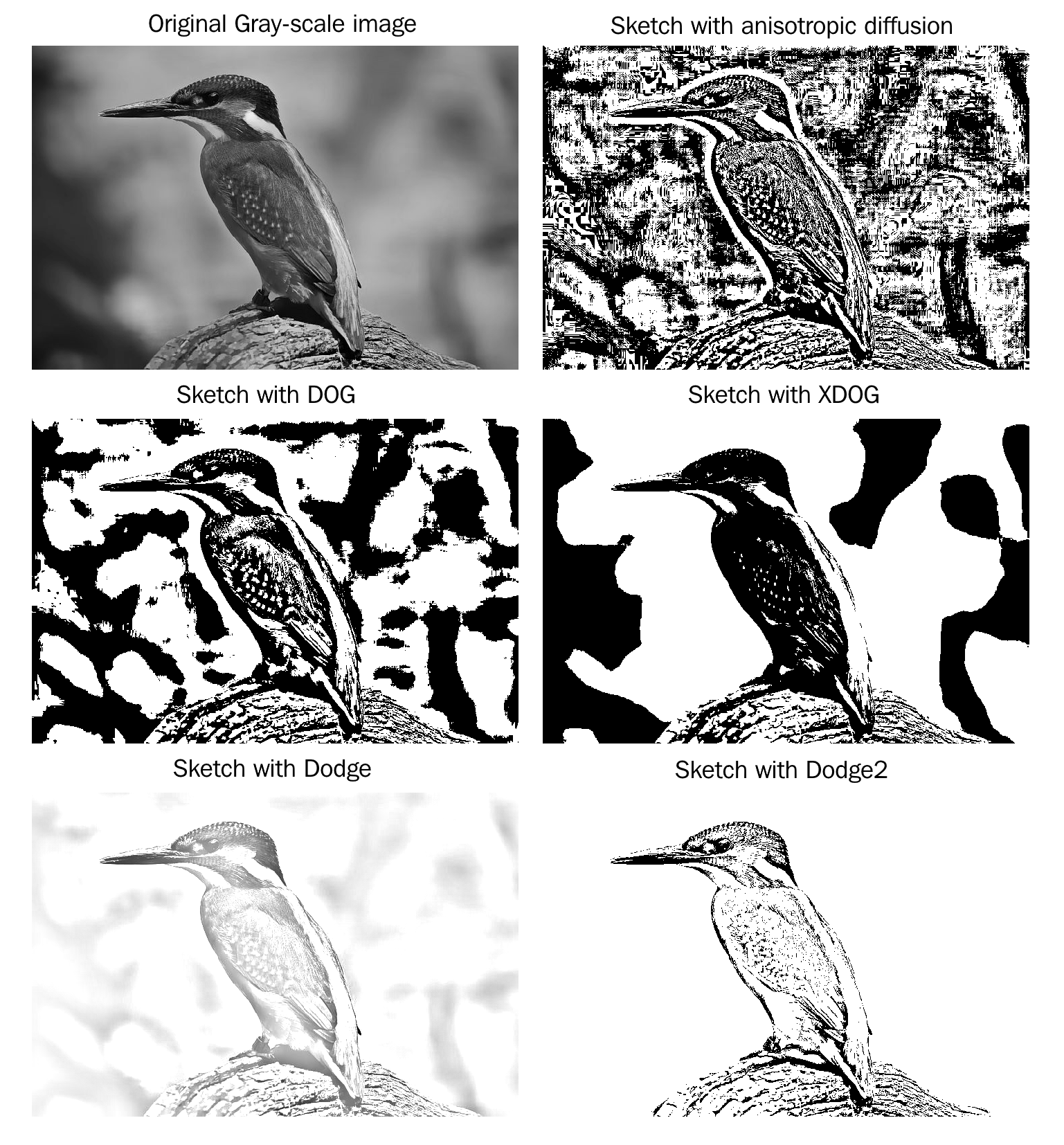
Producing sketches from images is all about detecting edges in images. In this recipe, you will learn how to use different techniques, including the difference of Gaussian (and its extended version, XDOG), anisotropic diffusion, and dodging (applying Gaussian blur + invert + thresholding), to obtain sketches from images.
Creating pencil sketches from images
Getting ready
The following libraries need to be imported first:
import numpy as np
from skimage.io import imread
from skimage.color import rgb2gray
from skimage import util
from skimage import img_as_float
import matplotlib.pylab as plt
from medpy.filter.smoothing import anisotropic_diffusion
from skimage.filters import gaussian, threshold_otsu
How to do it...
The following steps need to be performed:
- Define the normalize() function to implement min-max normalization in an image:
def normalize(img):
    return (img-np.min(img))/(np.max(img)-np.min(img))
- Implement the sketch() function that takes an image and the extracted edges as input:
def sketch(img, edges):
    output = np.multiply(img, edges)
    output[output>1]=1
    output[edges==1]=1
    return output
- Implement a function to extract the edges from an image with anisotropic diffusion:
def edges_with_anisotropic_diffusion(img, niter=100, kappa=10, gamma=0.1):
    output = img - anisotropic_diffusion(img, niter=niter, \
            kappa=kappa, gamma=gamma, voxelspacing=None, \
            option=1)
    output[output > 0] = 1
    output[output < 0] = 0
    return output
- Implement a function to extract the edges from an image with the dodge operation (there are two implementations):
def sketch_with_dodge(img):
 orig = img
 blur = gaussian(util.invert(img), sigma=20)
 result = blur / util.invert(orig)
 result[result>1] = 1
 result[orig==1] = 1
 return result

def edges_with_dodge2(img):
 img_blurred = gaussian(util.invert(img), sigma=5)
 output = np.divide(img, util.invert(img_blurred) + 0.001)
 output = normalize(output)
 thresh = threshold_otsu(output)
 output = output > thresh
 return output
- Implement a function to extract the edges from an image with a Difference of Gaussian (DOG) operation:
def edges_with_DOG(img, k = 200, gamma = 1):
    sigma = 0.5
    output = gaussian(img, sigma=sigma) - gamma*gaussian(img, \
                      sigma=k*sigma)
    output[output > 0] = 1
    output[output < 0] = 0
    return output
- Implement a function to produce sketches from an image with an Extended Difference of Gaussian (XDOG) operation:
def sketch_with_XDOG(image, epsilon=0.01):
    phi = 10
    difference = edges_with_DOG(image, 200, 0.98).astype(np.uint8)
    for i in range(0, len(difference)):
        for j in range(0, len(difference[0])):
            if difference[i][j] >= epsilon:
                difference[i][j] = 1
            else:
                ht = np.tanh(phi*(difference[i][j] - epsilon))
            difference[i][j] = 1 + ht
    difference = normalize(difference)
    return difference
If you run the preceding code and plot all of the input/output images, you will obtain an output like the following screenshot:

How it works...
As you can see from the previous section, many of the sketching techniques work by blurring the edges (for example, with Gaussian filter or diffusion) in the image and removing details to some extent and then subtracting the original image to get the sketch outlines.
The gaussian() function from the scikit-image filters module was used to blur the images.
The anisotropic_diffusion() function from the filter.smoothing module of the medpy library was used to find edges with anisotropic diffusion (a variational method).
The dodge operation divides (using np.divide()) the image by the inverted blurred image. This highlights the boldest edges in the image.
There's more...
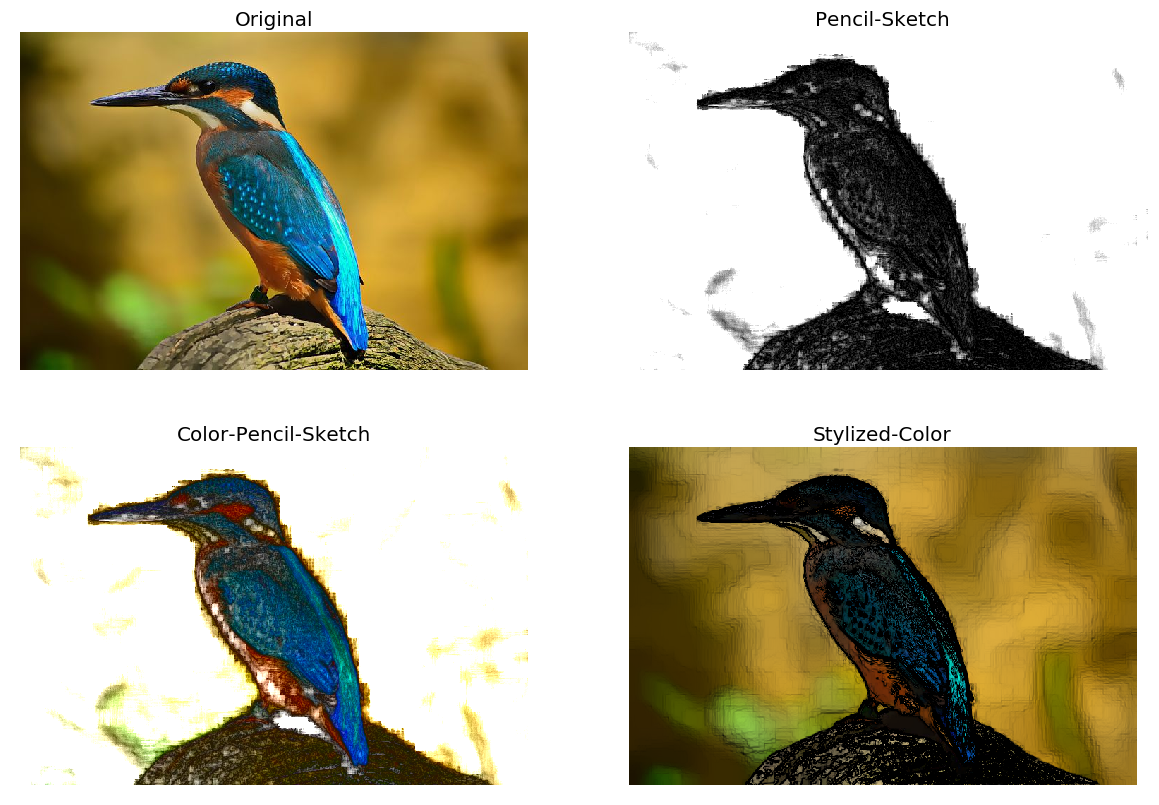
There are a few more edge detection techniques, such as Canny (with hysteresis thresholds), that you can try to produce sketches from images. You can try them on your own and compare the sketches obtained using different algorithms. Also, by using OpenCV-Python's pencilSketch() and sylization() functions, you can produce black and white and color pencil sketches, as well as watercolor-like stylized images, with the following few lines of code:
import cv2
import matplotlib.pylab as plt
src = cv2.imread('images/bird.png')
#dst = cv2.detailEnhance(src, sigma_s=10, sigma_r=0.15)
dst_sketch, dst_color_sketch = cv2.pencilSketch(src, sigma_s=50, sigma_r=0.05, shade_factor=0.05)
dst_water_color = cv2.stylization(src, sigma_s=50, sigma_r=0.05)
If you run this code and plot the images, you will get a diagram similar to the following screenshot:

See also
For more details, refer to the following link:


