In this recipe, you will learn how to create cartoonish flat-textured images from an image. Again, there is more than one way to do the same; here, we will learn how to do it with edge-preserving bilateral filters.
Creating cartoonish images
Getting ready
The following libraries need to be imported first:
import cv2
import numpy as np
import matplotlib.pylab as plt
How to do it...
For this recipe, we will be using the bilateralFilter() function from OpenCV-Python. We need to start by downsampling the image to create an image pyramid (you will see more of this in the next chapter), followed by repeated application of small bilateral filters (to remove unimportant details) and upsampling the image to its original size. Next, you need to apply the median blur (to flatten the texture) followed by masking the original image with the binary image obtained by adaptive thresholding. The following code demonstrates the steps:
- Read the input image and initialize the parameters to be used later:
img = plt.imread("images/bean.png")

num_down = 2 # number of downsampling steps
num_bilateral = 7 # number of bilateral filtering steps

w, h, _ = img.shape
- Use the Gaussian pyramid's downsampling to reduce the image size (and make the subsequent operations faster):
img_color = np.copy(img)
for _ in range(num_down):
 img_color = cv2.pyrDown(img_color)
- Apply bilateral filters (with a small diameter value) iteratively. The d parameter represents the diameter of the neighborhood for each pixel, where the sigmaColor and sigmaSpace parameters represent the filter sigma in the color and the coordinate spaces, respectively:
for _ in range(num_bilateral):
 img_color = cv2.bilateralFilter(img_color, d=9, sigmaColor=0.1, sigmaSpace=0.01)
- Use upsampling to enlarge the image to the original size:
for _ in range(num_down):
 img_color = cv2.pyrUp(img_color)
- Convert to the output image obtained from the last step and blur the image with the median filter:
img_gray = cv2.cvtColor(img, cv2.COLOR_RGB2GRAY)
img_blur = cv2.medianBlur(img_gray, 7)
- Detect and enhance the edges:
img_edge = cv2.adaptiveThreshold((255*img_blur).astype(np.uint8), \
            255, cv2.ADAPTIVE_THRESH_MEAN_C, cv2.THRESH_BINARY, \
            blockSize=9, C=2)
- Convert the grayscale edge image back into an RGB color image and compute bitwise AND with the RGB color image to get the final output cartoonish image:
img_edge = cv2.cvtColor(img_edge, cv2.COLOR_GRAY2RGB)
img_cartoon = cv2.bitwise_and(img_color, img_edge)
How it works...
As explained earlier, the bilateralFilter(), medianBlur(), adaptiveThreshold(), and bitwise_and() functions from OpenCV-Python were the key functions used to first remove weak edges, then convert into flat texture, and finally enhance the prominent edges in the image.
The bilateralFilter() function from OpenCV-Python was used to smooth the textures while keeping the edges fairly sharp:
- The higher the value of the sigmaColor parameter, the more the pixel colors in the neighborhood will be mixed together. This will produce larger areas of semi-equal color in the output image.
- The higher the value of the sigmaSpace parameter, the more the pixels with similar colors will influence each other.
The image was downsampled to create an image pyramid (you will see more of this in the next chapter).
Next, repeated application of small bilateral filters was used to remove unimportant details. A subsequent upsampling was used to resize the image to its original size.
Finally, medianBlur was applied (to flatten the texture) followed by masking the original image with the binary image obtained by adaptive thresholding.
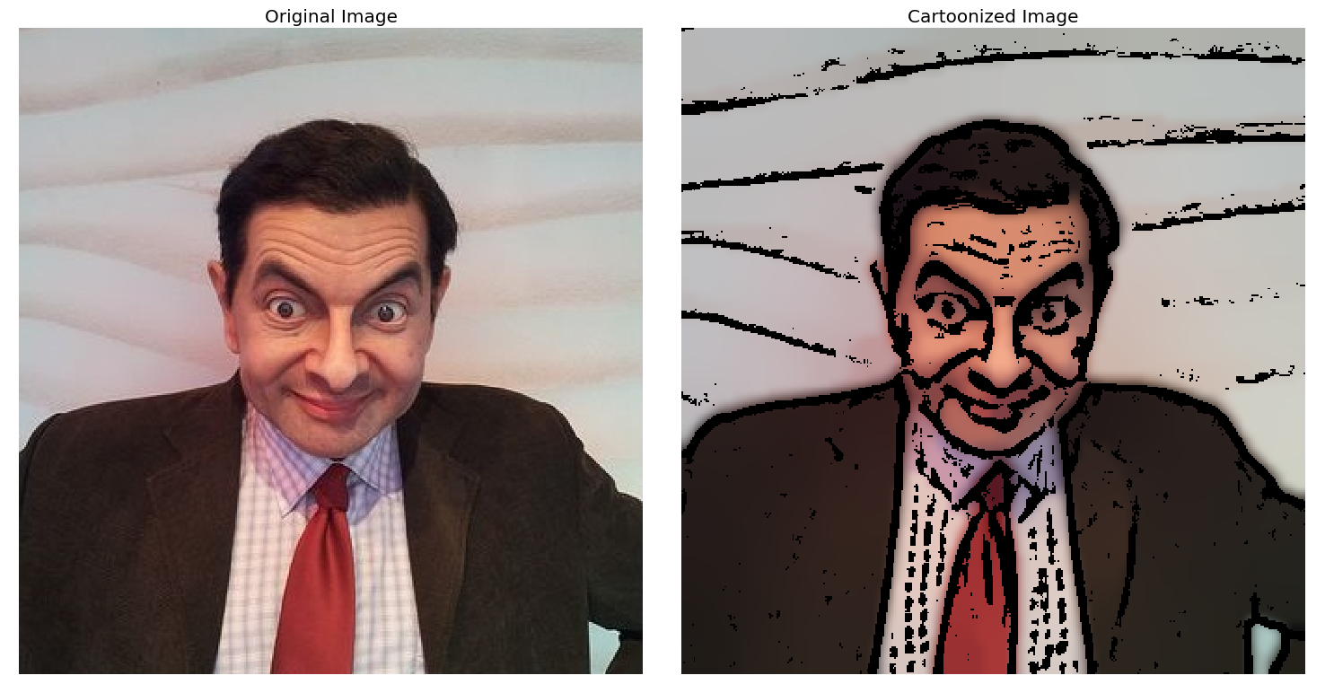
If you run the preceding code, you will get an output cartoonish image, as shown here:
There's more...
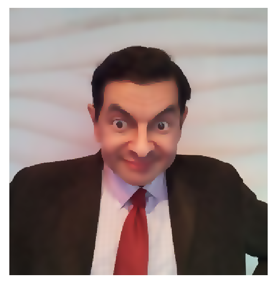
Play with the parameter values of the OpenCV functions to see the impact on the output image produced. Also, as mentioned earlier, there is more than one way to achieve the same effect. Try using anisotropic diffusion to obtain flat texture images. You should get an image like the following one (use the anisotropic_diffusion() function from the medpy library):
See also
For more details, refer to the following links:


