Point cloud data
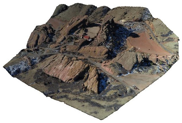
Remote sensing data can measure the Earth in two dimensions. But we can also use remote sensing to measure the Earth and things on it in three dimensions using point cloud data. Point cloud data are collections of discrete points with horizontal coordinates represented by X and Y values and a vertical coordinate represented by a Z value. These points are collected in a variety of ways, including lasers (as in the case of lidar data), sound (which is commonly used for mapping the seafloor but can also be used on land), stereoscopic imagery, radio waves (such as radar), or “structure-in-motion” data, where a single geo-located camera is used to collect overlapping images to estimate the 3D structure of a scene. Point cloud data can be mapped relative to any origin and is not necessarily dependent on GPS like other types of geospatial data. This feature allows it to be used to map indoor spaces, as well as outdoor spaces. Point cloud data can also be colorized for visualization using color photography or video for creating immersive 3D models, as shown in the following colorized point cloud of Red Rocks, Colorado, USA:

Figure 1.9 – A colorized lidar point cloud of Red Rocks, Colorado, USA, which creates a photorealistic 3D model
Point cloud data is the most common way to create elevation data that can be turned into a gridded format. This is called a Digital Elevation Model (DEM). A DEM is a three-dimensional representation of a planet’s terrain. In the context of this book, this planet is the Earth. The history of digital elevation models is far less complicated than remotely-sensed imagery but no less significant. Before computers, representations of elevation data were limited to topographic maps created through traditional land surveys. The technology existed to create three-dimensional models from stereoscopic images or physical models from materials such as clay or wood, but these approaches were not widely used for geography.
The concept of digital elevation models came about in 1986 when the French space agency, Centre National d’études Spatiales (CNES) or National Center for the Study of Space, launched its SPOT-1 satellite, which included a stereoscopic radar. This system created the first usable DEM. Several other US and European satellites followed this model with similar missions.
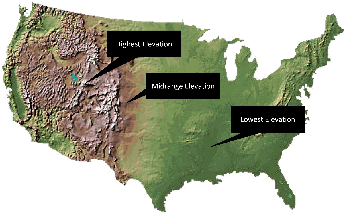
In February 2000, the space shuttle Endeavour conducted the Shuttle Radar Topography Mission (SRTM), which collected elevation data of over 80% of the Earth’s surface using a special radar antenna configuration that allowed a single pass. This model was surpassed in 2009 by the joint US and Japanese mission, which used the Advanced Spaceborne Thermal Emission and Reflection Radiometer (ASTER) sensor aboard NASA’s Terra satellite. This system captured 99% of the Earth’s surface but has proven to have minor data issues. Since the Space Shuttle’s orbit did not cross the Earth’s poles, it did not capture the entire surface. SRTM remains the gold standard. The following figure from the USGS (https://www.usgs.gov/media/images/national-elevation-dataset) shows a colorized DEM known as a hill shade. Greener areas are at lower elevations, while yellow and brown areas are at mid-range to high elevations:

Figure 1.10 – An example of a DEM using colors and hill shade shadows to create a natural-looking representation of elevation
Recently, more ambitious attempts at a worldwide elevation dataset are underway in the form of the TerraSAR-X and TanDEM-X satellites, which were launched by Germany in 2007 and 2010, respectively. These two radar elevation satellites worked together to produce a global DEM called WorldDEM, which was released on April 15, 2014. This dataset has a relative accuracy of 2 meters and an absolute accuracy of 4 meters.


