Search icon CANCEL
Subscription
0
Cart icon
Your Cart (0 item)
Close icon
You have no products in your basket yet
Save more on your purchases! discount-offer-chevron-icon
Savings automatically calculated. No voucher code required.
Arrow left icon
Explore Products
Best Sellers
New Releases
Books
Videos
Audiobooks
Learning Hub
Newsletter Hub
Free Learning
Arrow right icon
timer SALE ENDS IN
0 Days
:
00 Hours
:
00 Minutes
:
00 Seconds
Arrow up icon
GO TO TOP
Deep Learning Essentials

You're reading from   Deep Learning Essentials Your hands-on guide to the fundamentals of deep learning and neural network modeling

Arrow left icon
Product type Paperback
Published in Jan 2018
Publisher Packt
ISBN-13 9781785880360
Length 284 pages
Edition 1st Edition
Languages
Tools
Arrow right icon
Authors (3):
Arrow left icon
Wei Di Wei Di
Author Profile Icon Wei Di
Wei Di
Anurag Bhardwaj Anurag Bhardwaj
Author Profile Icon Anurag Bhardwaj
Anurag Bhardwaj
Jianing Wei Jianing Wei
Author Profile Icon Jianing Wei
Jianing Wei
Arrow right icon
View More author details
Toc

Table of Contents (12) Chapters Close

Preface 1. Why Deep Learning? 2. Getting Yourself Ready for Deep Learning FREE CHAPTER 3. Getting Started with Neural Networks 4. Deep Learning in Computer Vision 5. NLP - Vector Representation 6. Advanced Natural Language Processing 7. Multimodality 8. Deep Reinforcement Learning 9. Deep Learning Hacks 10. Deep Learning Trends 11. Other Books You May Enjoy

The motivation of deep architecture

The depth of the architecture refers to the number of levels of the composition of non-linear operations in the function learned. These operations include weighted sum, product, a single neuron, kernel, and so on. Most current learning algorithms correspond to shallow architectures that have only 1, 2, or 3 levels. The following table shows some examples of both shallow and deep algorithms:

Levels

Example

Group

1-layer

Logistic regression,

Maximum Entropy Classifier

Perceptron, Linear SVM

Linear classifier

2-layers

Multi-layer Perceptron,

SVMs with kernels

Decision trees

Universal approximator

3 or more layers

Deep learning

Boosted decision trees

Compact universal approximator

There are mainly two viewpoints of understanding the deep architecture of deep learning algorithms: the neural point view and the feature representation view. We will talk about each of them. Both of them may come from different origins, but together they can help us to better understand the mechanisms and advantages deep learning has.

The neural viewpoint

From a neural viewpoint, an architecture for learning is biologically inspired. The human brain has deep architecture, in which the cortex seems to have a generic learning approach. A given input is perceived at multiple levels of abstraction. Each level corresponds to a different area of the cortex. We process information in hierarchical ways, with multi-level transformation and representation. Therefore, we learn simple concepts first then compose them together. This structure of understanding can be seen clearly in a human’s vision system. As shown in the following figure, Signal path from the retina to human lateral occipital cortex (LOC), which finally recognizes the object, the ventral visual cortex comprises a set of areas that process images in increasingly more abstract ways, from edges, corners and contours, shapes, object parts to object, allowing us to learn, recognize, and categorize three-dimensional objects from arbitrary two-dimensional views:

The signal path from the retina to human lateral occipital cortex (LOC), which finally recognizes the object. Figure credit to Jonas Kubilius (https://neuwritesd.files.wordpress.com/2015/10/visual_stream_small.png)

The representation viewpoint

For most traditional machine learning algorithms, their performance depends heavily on the representation of the data they are given. Therefore, domain prior knowledge, feature engineering, and feature selection are critical to the performance of the output. But hand-crafted features lack the flexibility of applying to different scenarios or application areas. Also, they are not data-driven and cannot adapt to new data or information comes in. In the past, it has been noticed that a lot of AI tasks could be solved by using a simple machine learning algorithm on the condition that the right set of features for the task are extracted or designed. For example, an estimate of the size of a speaker’s vocal tract is considered a useful feature, as it’s a strong clue as to whether the speaker is a man, woman, or child. Unfortunately, for many tasks, and for various input formats, for example, image, video, audio, and text, it is very difficult to know what kind of features should be extracted, let alone their generalization ability for other tasks that are beyond the current application. Manually designing features for a complex task requires a great deal of domain understanding, time, and effort. Sometimes, it can take decades for an entire community of researchers to make progress in this area. If one looks back at the area of computer vision, for over a decade researchers have been stuck because of the limitations of the available feature extraction approaches (SIFT, HOG, and so on). A lot of work back then involved trying to design complicated machine learning schema given such base features, and the progress was very slow, especially for large-scale complicated problems, such as recognizing 1000 objects from images. This is a strong motivation for designing flexible and automated feature representation approaches.

One solution to this problem is to use the data driven type of approach, such as machine learning to discover the representation. Such representation can represent the mapping from representation to output (supervised), or simply representation itself (unsupervised). This approach is known as representation learning. Learned representations often result in much better performance as compared to what can be obtained with hand-designed representations. This also allows AI systems to rapidly adapt to new areas, without much human intervention. Also, it may take more time and effort from a whole community to hand-craft and design features. While with a representation learning algorithm, we can discover a good set of features for a simple task in minutes or a complex task in hours to months.

This is where deep learning comes to the rescue. Deep learning can be thought of as representation learning, whereas feature extraction happens automatically when the deep architecture is trying to process the data, learning, and understanding the mapping between the input and the output. This brings significant improvements in accuracy and flexibility since human designed feature/feature extraction lacks accuracy and generalization ability.

In addition to this automated feature learning, the learned representations are both distributed and with a hierarchical structure. Such successful training of intermediate representations helps feature sharing and abstraction across different tasks.

The following figure shows its relationship as compared to other types of machine learning algorithms. In the next section, we will explain why these characteristics (distributed and hierarchical) are important:

A Venn diagram showing how deep learning is a kind of representation learning

Distributed feature representation

A distributed representation is dense, whereas each of the learned concepts is represented by multiple neurons simultaneously, and each neuron represents more than one concept. In other words, input data is represented on multiple, interdependent layers, each describing data at different levels of scale or abstraction. Therefore, the representation is distributed across various layers and multiple neurons. In this way, two types of information are captured by the network topology. On the one hand, for each neuron, it must represent something, so this becomes a local representation. On the other hand, so-called distribution means a map of the graph is built through the topology, and there exists a many-to-many relationship between these local representations. Such connections capture the interaction and mutual relationship when using local concepts and neurons to represent the whole. Such representation has the potential to capture exponentially more variations than local ones with the same number of free parameters. In other words, they can generalize non-locally to unseen regions. They hence offer the potential for better generalization because learning theory shows that the number of examples needed (to achieve the desired degree of generalization performance) to tune O (B) effective degrees of freedom is O (B). This is referred to as the power of distributed representation as compared to local representation (http://www.iro.umontreal.ca/~pift6266/H10/notes/mlintro.html).

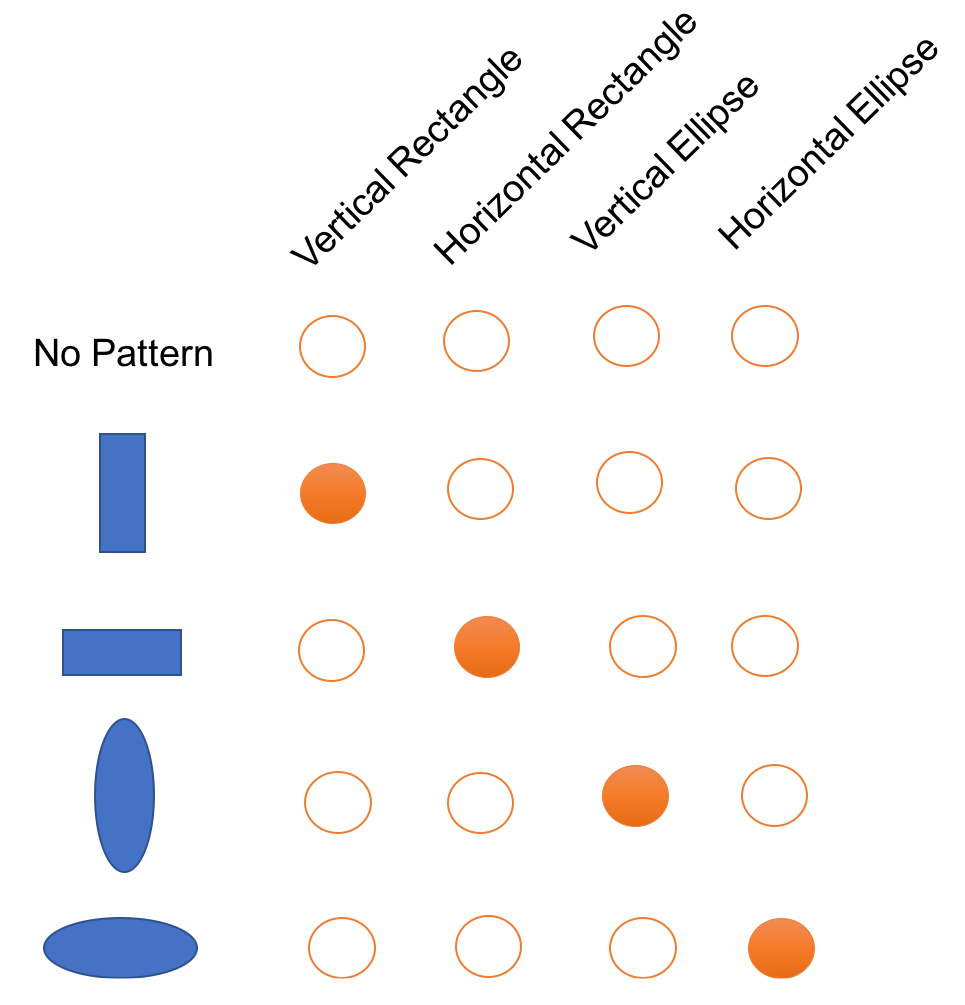
An easy way to understand the example is as follows. Suppose we need to represent three words, one can use the traditional one-hot encoding (length N), which is commonly used in NLP. Then at most, we can represent N words. The localist models are very inefficient whenever the data has componential structure:

One-hot encoding

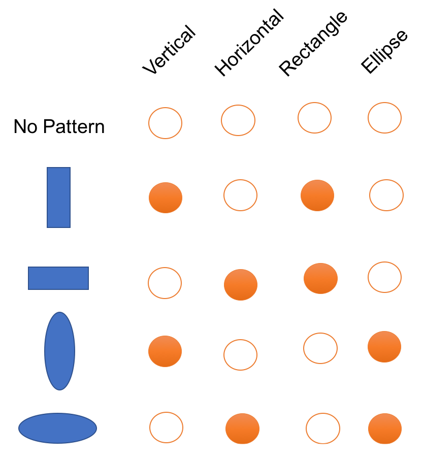
A distributed representation of a set of shapes would look like this:

Distributed representation

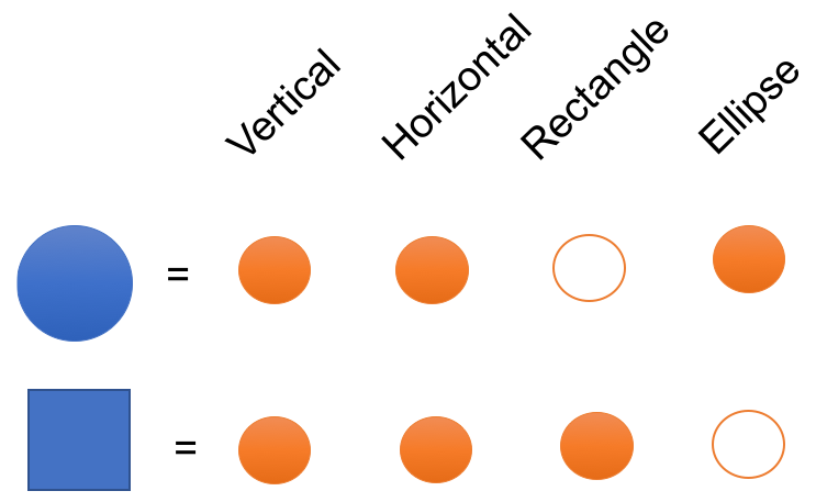
If we wanted to represent a new shape with a sparse representation, such as one-hot-encoding, we would have to increase the dimensionality. But what’s nice about a distributed representation is we may be able to represent a new shape with the existing dimensionality. An example using the previous example is as follows:

Representing new concepts using distributed representation

Therefore, non-mutually exclusive features/attributes create a combinatorially large set of distinguishable configurations and the number of distinguishable regions grows almost exponentially with the number of parameters.

One more concept we need to clarify is the difference between distributed and distributional. Distributed is represented as continuous activation levels in a number of elements, for example, a dense word embedding, as opposed to one-hot encoding vectors.

On the other hand, distributional is represented by contexts of use. For example, Word2Vec is distributional, but so are count-based word vectors, as we use the contexts of the word to model the meaning.

Hierarchical feature representation

The learnt features capture both local and inter-relationships for the data as a whole, it is not only the learnt features that are distributed, the representations also come hierarchically structured. The previous figure, Comparing deep and shallow architecture. It can be seen that shallow architecture has a more flat topology, while deep architecture has many layers of hierarchical topology compares the typical structure of shallow versus deep architectures, where we can see that the shallow architecture often has a flat structure with one layer at most, whereas the deep architecture structures have multiple layers, and lower layers are composited that serve as input to the higher layer. The following figure uses a more concrete example to show what information has been learned through layers of the hierarchy.

As shown in the image, the lower layer focuses on edges or colors, while higher layers often focus more on patches, curves, and shapes. Such representation effectively captures part-and-whole relationships from various granularity and naturally addresses multi-task problems, for example, edge detection or part recognition. The lower layer often represents the basic and fundamental information that can be used for many distinct tasks in a wide variety of domains. For example, Deep Belief networks have been successfully used to learn high-level structures in a wide variety of domains, including handwritten digits and human motion capture data. The hierarchical structure of representation mimics the human understanding of concepts, that is, learning simple concepts first and then successfully building up more complex concepts by composing the simpler ones together. It is also easier to monitor what is being learnt and to guide the machine to better subspaces. If one treats each neuron as a feature detector, then deep architectures can be seen as consisting of feature detector units arranged in layers. Lower layers detect simple features and feed into higher layers, which in turn detect more complex features. If the feature is detected, the responsible unit or units generate large activations, which can be picked up by the later classifier stages as a good indicator that the class is present:

Illustration of hierarchical features learned from a deep learning algorithm. Image by Honglak Lee and colleagues as published in Convolutional Deep Belief Networks for Scalable Unsupervised Learning of Hierarchical Representations, 2009

The above figure illustrates that each feature can be thought of as a detector, which tries to the detector a particular feature (blob, edges, nose, or eye) on the input image.

lock icon The rest of the chapter is locked
Register for a free Packt account to unlock a world of extra content!
A free Packt account unlocks extra newsletters, articles, discounted offers, and much more. Start advancing your knowledge today.
Unlock this book and the full library FREE for 7 days
Get unlimited access to 7000+ expert-authored eBooks and videos courses covering every tech area you can think of
Renews at $19.99/month. Cancel anytime
Banner background image