Unifying batch and streaming data processing
One of the core features that Beam offers is the portability of data processing pipelines between batch and streaming processing. This began around 2004, with the famous white paper, MapReduce: Simplified Data Processing on Large Clusters. The idea behind MapReduce is quite simple: divide a complex computation into several parts, each of which consists of two functions – Map and Reduce – and apply these functions on a large scale using clusters of commodity hardware. The simplicity of the two building blocks gives rise to quite simple requirements in terms of fault tolerance, which is essential for any large distributed system.
Details of this system can be easily found online and are out of the scope of this book. We reference it here to demonstrate how and why data processing systems evolved from this moment on. The greatest benefit – massive parallel processing of data on clusters of computers that fail – is what enabled the cost-effectiveness of these large computations and finally led to the development of deep learning applications and other computationally intensive approaches.
The approach has two major drawbacks:
- Complex algorithms typically require a very difficult decomposition into
MapandReducefunctions, the chaining of multiple stages, and so on. - The latency of data processing is very high due to the fact that all data has to be reprocessed from scratch and no continuous updates are possible.
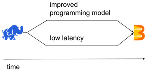
At first, both of these drawbacks were addressed by different systems. Therefore, batch systems with higher-level primitives (such as joins and groupings) came out (for example, Apache Spark), while, at the same time, different systems tailored to low-latency processing came out (for example, Apache Storm). The evolution of these systems can be illustrated as follows:

Figure 1.14 – Evolving from Apache Hadoop to Apache Beam
Apache Beam was the first model to unify both of these evolving paths into a single model, and it was targeted at both low-latency and advanced programming models. This was enabled by a simple (but very crucial) insight: batch semantics can be defined using streaming semantics (this statement is often rephrased as batch is a special case of streaming). Let's see how exactly this was achieved.
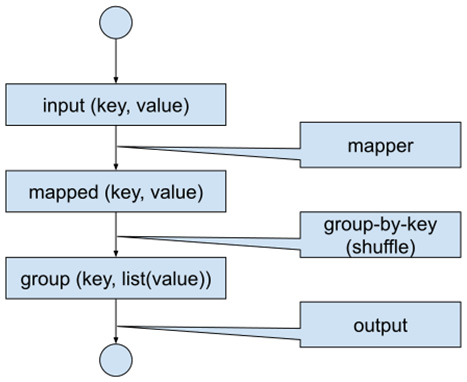
Due to the described simplicity of parallelizing a chain of MapReduce operations, practically all batch systems targeted at improving the programming model were defining high-level abstractions, which then, in turn, translated to low-level MapReduce-like operations. Therefore, we can focus on the simple MapReduce paradigm for the batch case, which works as follows:

Figure 1.15 – Batch data flow
For clarity, we will briefly describe how the processing works. Each input record is fed into the Map function, producing possibly multiple key-value pairs. Each record with the same key is then grouped together and fed into the Reduce function, which (for the given key and list of values) produces final outputs.
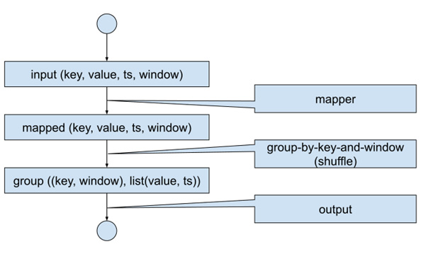
As we have seen in this chapter, in the case of streaming semantics, there are two more things to worry about: an event time of a stream element, and a window function that assigns these elements into windows (tumbling, sliding, session). Therefore, if we extend the batch processing with the event time of each key-value pair and define a sensible default window, we get the situation depicted in Figure 1.16.
Each element is now equipped with a default timestamp (ts) and a default window:

Figure 1.16 – Batch data flow with streaming semantics
We have to define sensible defaults for the timestamp and window. The timestamp can be chosen at a fixed value (typically, either the timestamp of the start of the batch computation, or –infinity), and the default window is the global window. The reason why there is no meaningful option other than to put all of the elements into a single window is that we must extend the GroupByKey operation in classical batch mode to GroupByKeyAndWindow to fulfill the streaming constraint that the state is bound to the window. In order to be able to derive the batch semantics from the streaming one, we see that the default window must assign the complete input to a single window (the global window).
Last but not least, we have to deal with how the event time moves in our streaming pipeline-running batch workflow. As we have seen, streaming processing uses watermarks to mark the progress of the event time. Batch semantics have no order in the input dataset (or in how the input data set is processed), therefore, we need to move the watermark from –infinity at the beginning and during the job to +infinity once the job completes (more exactly, when the job finishes reducing the last key).
Important note
Under special circumstances, it is possible to smoothly advance the event time watermark, even in the case of batch processing. We will learn more about this topic when we explore the stateful processing of time series data.
To sum this up, we can see that we can derive batch semantics from streaming semantics by performing the following:
- Assigning a fixed timestamp to all input key-value pairs.
- Assigning all input key-value pairs to the global window.
- Moving the watermark from –inf to +inf in one hop once all the data is processed
So, the unified approach of Beam comes from the following logic:
Code your pipeline as a streaming pipeline then run it in both a batch and streaming fashion.
There are some cases where an exception to this rule makes sense, but every time you code a batch-only pipeline in Beam, you should take one step back and think if it is really what you want.


