Assumptions of Regression Analysis
Due to the parametric nature of linear regression analysis, the method makes certain assumptions about the data it analyzes. When these assumptions are not met, the results of the regression analysis may be misleading to say the least. It is, therefore, necessary to check any analysis work to ensure the regression assumptions are not violated.
Let's review the main assumptions of linear regression analysis that we must ensure are met in order to develop a good model:
- The relationship between the dependent and independent variables must be linear and additive.
This means that the relationship must be of the straight-line type, and if there are many independent variables involved, thus multiple linear regression, the weighted sum of these independent variables must be able to explain the variability in the dependent variable.
- The residual terms (ϵi) must be normally distributed. This is so that the standard error of estimate is calculated correctly. This standard error of estimate statistic is used to calculate t-values, which, in turn, are used to make statistical significance decisions. So, if the standard error of estimate is wrong, the t-values will be wrong and so are the statistical significance decisions that follow on from the p-values. The t-values that are calculated using the standard error of estimate are also used to construct confidence intervals for the population regression parameters. If the standard error is wrong, then the confidence intervals will be wrong as well.
- The residual terms (ϵi) must have constant variance (homoskedasticity). When this is not the case, we have the heteroskedasticity problem. This point refers to the variance of the residual terms. It is assumed to be constant. We assume that each data point in our regression analysis contributes equal explanation to the variability we are seeking to model. If some data points contribute more explanation than others, our regression line will be pulled toward the points with more information. The data points will not be equally scattered around our regression line. The error (variance) about the regression line, in that case, will not be constant.
- The residual terms (ϵi) must not be correlated. When there is correlation in the residual terms, we have the problem known as autocorrelation. Knowing one residual term, must not give us any information about what the next residual term will be. Residual terms that are autocorrelated are unlikely to have a normal distribution.
- There must not be correlation among the independent variables. When the independent variables are correlated among themselves, we have a problem called multicollinearity. This would lead to developing a model with coefficients that have values that depend on the presence of other independent variables. In other words, we will have a model that will change drastically should a particular independent variable be dropped from the model for example. A model like that will be inaccurate.
Activity 2.02: Fitting a Multiple Log-Linear Regression Model
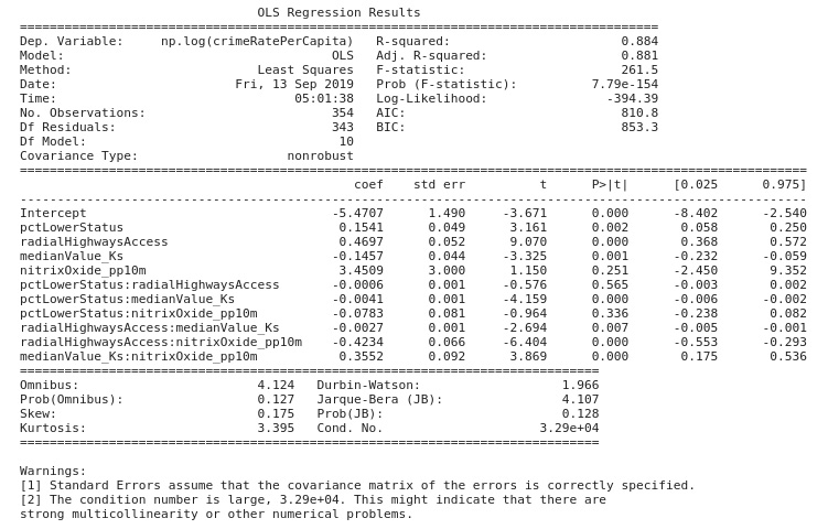
A log-linear regression model you developed earlier was able to explain about 24% of the variability in the transformed crime rate per capita variable. You are now asked to develop a log-linear multiple regression model that will likely explain 80% or more of the variability in the transformed dependent variable. You should use independent variables from the Boston Housing dataset that have a correlation coefficient of 0.4 or more.
You are also encouraged to include the interaction of these variables to order two in your model. You should produce graphs and data that show that your model satisfies the assumptions of linear regression.
The steps are as follows:
- Define a linear regression model and assign it to a variable. Remember to use the
logfunction to transform the dependent variable in the formula string, and also include more than one independent variable in your analysis. - Call the
fitmethod of the model instance and assign the results of the method to a new variable. - Print a summary of the results and analyze your model.
Your output should appear as shown:

Figure 2.19: Expected OLS results
Note
The solution to this activity can be found here: https://packt.live/2GbJloz.


