Search icon CANCEL
Subscription
0
Cart icon
Your Cart (0 item)
Close icon
You have no products in your basket yet
Save more on your purchases! discount-offer-chevron-icon
Savings automatically calculated. No voucher code required.
Arrow left icon
Explore Products
Best Sellers
New Releases
Books
Videos
Audiobooks
Learning Hub
Newsletter Hub
Free Learning
Arrow right icon
timer SALE ENDS IN
0 Days
:
00 Hours
:
00 Minutes
:
00 Seconds
Arrow up icon
GO TO TOP
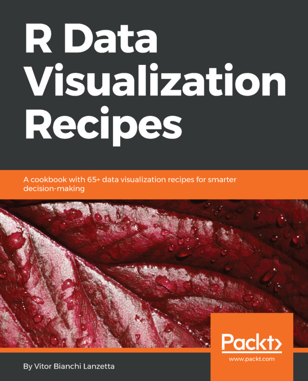
R Data Visualization Recipes

You're reading from   R Data Visualization Recipes A cookbook with 65+ data visualization recipes for smarter decision-making

Arrow left icon
Product type Paperback
Published in Nov 2017
Publisher Packt
ISBN-13 9781788398312
Length 366 pages
Edition 1st Edition
Languages
Tools
Arrow right icon
Author (1):
Arrow left icon
Vitor Bianchi Lanzetta Vitor Bianchi Lanzetta
Author Profile Icon Vitor Bianchi Lanzetta
Vitor Bianchi Lanzetta
Arrow right icon
View More author details
Toc

Table of Contents (13) Chapters Close

Preface 1. Installation and Introduction FREE CHAPTER 2. Plotting Two Continuous Variables 3. Plotting a Discrete Predictor and a Continuous Response 4. Plotting One Variable 5. Making Other Bivariate Plots 6. Creating Maps 7. Faceting 8. Designing Three-Dimensional Plots 9. Using Theming Packages 10. Designing More Specialized Plots 11. Making Interactive Plots 12. Building Shiny Dashboards

Plotting a high quality faceted bar graph


To create publish-quality faceted bar graphs is not that different from creating publish-quality regular bar plots. This recipe will follow the usual steps we had been following until now: grow axes, make labels account full names, and resize texts. Besides, this changes, recipe will also adjust facet labels and colors in general.

Another cool thing is to do whenever your x and fill aesthetics are matching is to set legends to replace the x axis title. This recipe will also demonstrate this.

How to do it...

We proceed with plotting a high quality faceted bar graph:

  1. Draw a basic faceted bar graph to work as the departure point:
> library(ggplot2)
> base <- ggplot(data = as.data.frame(Titanic), 
                aes(x = Survived)) + 
   geom_bar(aes(fill = Survived, weight = Freq), colour = 'black', width = 1) + 
   facet_grid(Sex ~ Age) + theme_bw()
> h1

The base object looks like the following illustration (Figure 7.10):

Figure 7.10 - Starting...

lock icon The rest of the chapter is locked
Register for a free Packt account to unlock a world of extra content!
A free Packt account unlocks extra newsletters, articles, discounted offers, and much more. Start advancing your knowledge today.
Unlock this book and the full library FREE for 7 days
Get unlimited access to 7000+ expert-authored eBooks and videos courses covering every tech area you can think of
Renews at $19.99/month. Cancel anytime
Banner background image