
Different labels appear in a variable with different frequencies. Some categories of a variable appear a lot, that is, they are very common among the observations, whereas other categories appear only in a few observations. In fact, categorical variables often contain a few dominant labels that account for the majority of the observations and a large number of labels that appear only seldom. Categories that appear in a tiny proportion of the observations are rare. Typically, we consider a label to be rare when it appears in less than 5% or 1% of the population. In this recipe, we will learn how to identify infrequent labels in a categorical variable.
Pinpointing rare categories in categorical variables
Getting ready
To follow along with this recipe, download the Car Evaluation dataset from the UCI Machine Learning Repository by following the instructions in the Technical requirements section of this chapter.
How to do it...
Let's begin by importing the necessary libraries and getting the data ready:
- Import the required Python libraries:
import pandas as pd
import matplotlib.pyplot as plt
- Let's load the Car Evaluation dataset, add the column names, and display the first five rows:
data = pd.read_csv('car.data', header=None)
data.columns = ['buying', 'maint', 'doors', 'persons', 'lug_boot', 'safety', 'class']
data.head()
We get the following output when the code is executed from a Jupyter Notebook:
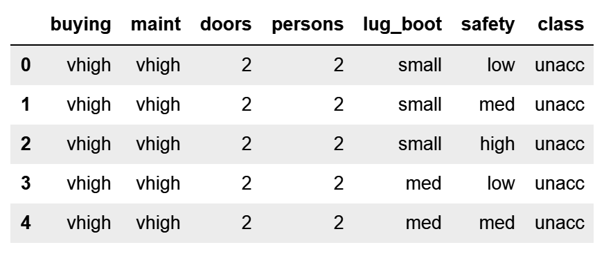
By default, pandas read_csv() uses the first row of the data as the column names. If the column names are not part of the raw data, we need to specifically tell pandas not to assign the column names by adding the header = None argument.
- Let's display the unique categories of the variable class:
data['class'].unique()
We can see the unique values of class in the following output:
array(['unacc', 'acc', 'vgood', 'good'], dtype=object)
- Let's calculate the number of cars per category of the class variable and then divide them by the total number of cars in the dataset to obtain the percentage of cars per category. Then, we'll print the result:
label_freq = data['class'].value_counts() / len(data)
print(label_freq)
The output of the preceding code block is a pandas Series, with the percentage of cars per category expressed as decimals:
- Let's make a bar plot showing the frequency of each category and highlight the 5% mark with a red line:
fig = label_freq.sort_values(ascending=False).plot.bar()
fig.axhline(y=0.05, color='red')
fig.set_ylabel('percentage of cars within each category')
fig.set_xlabel('Variable: class')
fig.set_title('Identifying Rare Categories')
plt.show()
The following is the output of the preceding block code:
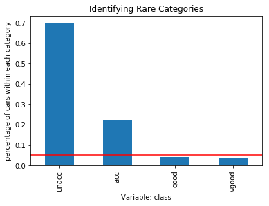
The good and vgood categories are present in less than 5% of cars, as indicated by the red line in the preceding plot.
How it works...
In this recipe, we quantified and plotted the percentage of observations per category, that is, the category frequency in a categorical variable of a publicly available dataset.
To load the data, we used pandas read_csv() and set the header argument to None, since the column names were not part of the raw data. Next, we added the column names manually by passing the variable names as a list to the columns attribute of the dataframe.
To determine the frequency of each category in the class variable, we counted the number of cars per category using pandas value_counts() and divided the result by the total cars in the dataset, which is determined with the Python built-in len method. Python's len method counted the number of rows in the dataframe. We captured the returned percentage of cars per category, expressed as decimals, in the label_freq variable.
To make a plot of the category frequency, we sorted the categories in label_freq from that of most cars to that of the fewest cars using the pandas sort_values() method. Next, we used plot.bar() to produce a bar plot. With axhline(), from Matplotlib, we added a horizontal red line at the height of 0.05 to indicate the 5% percentage limit, under which we considered a category as rare. We added x and y labels and a title with plt.xlabel(), plt.ylabel(), and plt.title() from Matplotlib.