Understanding linear algebra

Linear algebra is a key branch of mathematics. An understanding of linear algebra is crucial for deep learning, that is, neural networks. Throughout this chapter, we will go through the key and fundamental linear algebra prerequisites. Linear Algebra deals with linear systems of equations. Instead of working with scalars, we start working with matrices and vectors. Using linear algebra, we can describe complicated operations in deep learning.

Environment setup

Before we jump into the field of mathematics and its properties, it's essential for us to set up the development environment as it will provide us settings to execute the concepts we learn, meaning installing the compiler, dependencies, and IDE (Integrated Development Environment) to run our code base.

Setting up the Python environment in Pycharm

It is best to use an IDE like Pycharm to edit Python code as it provides development tools and built-in coding assistance. Code inspection makes coding and debugging faster and simpler, ensuring that you focus on the end goal of learning maths for neural networks.

The following steps show you how to set up local Python environment in Pycharm:

1. Go to Preferences and verify that the TensorFlow library is installed. If not, follow the instructions at https://www.tensorflow.org/install/ to install TensorFlow:

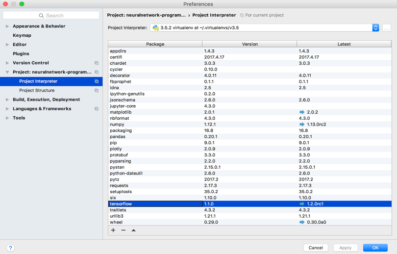
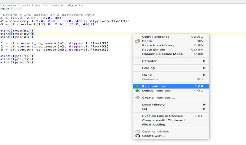
2. Keep the default options of TensorFlow and click on OK.
3. Finally, right-click on the source file and click on Run 'matrices':

Linear algebra structures

In the following section, we will describe the fundamental structures of linear algebra.

Scalars, vectors, and matrices

Scalars, vectors, and matrices are the fundamental objects of mathematics. Basic definitions are listed as follows:

• Scalar is represented by a single number or numerical value called magnitude.
• Vector is an array of numbers assembled in order. A unique index identifies each number. Vector represents a point in space, with each element giving the coordinate along a different axis.
• Matrices is a two-dimensional array of numbers where each number is identified using two indices (i, j).

Tensors

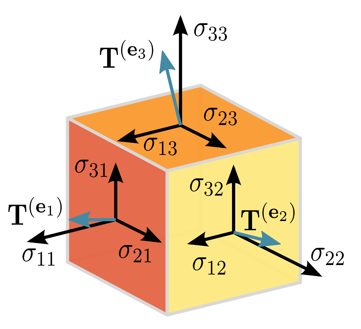
An array of numbers with a variable number of axes is known as a tensor. For example, for three axes, it is identified using three indices (i, j, k). 

The following image summaries a tensor, it describes a second-order tensor object. In a three-dimensional Cartesian coordinate system, tensor components will form the matrix:

      

Note

Image reference is taken from tensor wiki https://en.wikipedia.org/wiki/Tensor

Operations

The following topics will describe the various operations of linear algebra.

Vectors

The Normfunction is used to get the size of the vector; the norm of a vector x measures the distance from the origin to the point x. It is also known as the

norm, where p=2 is known as the Euclidean norm.

The following example shows you how to calculate the

norm of a given vector:

import tensorflow as tf

vector = tf.constant([[4,5,6]], dtype=tf.float32)
eucNorm = tf.norm(vector, ord="euclidean")

with tf.Session() as sess:
print(sess.run(eucNorm))

The output of the listing is 8.77496.

Matrices

A matrix is a two-dimensional array of numbers where each element is identified by two indices instead of just one. If a real matrix X has a height of m and a width of n, then we say that X ∈ Rm × n. Here, R is a set of real numbers.

The following example shows how different matrices are converted to tensor objects:

# convert matrices to tensor objects
import numpy as np
import tensorflow as tf

# create a 2x2 matrix in various forms
matrix1 = [[1.0, 2.0], [3.0, 40]]
matrix2 = np.array([[1.0, 2.0], [3.0, 40]], dtype=np.float32)
matrix3 = tf.constant([[1.0, 2.0], [3.0, 40]])

print(type(matrix1))
print(type(matrix2))
print(type(matrix3))

tensorForM1 = tf.convert_to_tensor(matrix1, dtype=tf.float32)
tensorForM2 = tf.convert_to_tensor(matrix2, dtype=tf.float32)
tensorForM3 = tf.convert_to_tensor(matrix3, dtype=tf.float32)

print(type(tensorForM1))
print(type(tensorForM2))
print(type(tensorForM3))

The output of the listing is shown in the following code:

<class 'list'>
<class 'numpy.ndarray'>
<class 'tensorflow.python.framework.ops.Tensor'>
<class 'tensorflow.python.framework.ops.Tensor'>
<class 'tensorflow.python.framework.ops.Tensor'>
<class 'tensorflow.python.framework.ops.Tensor'>

Matrix multiplication

Matrix multiplication of matrices A and B is a third matrix, C:

C = AB

The element-wise product of matrices is called a Hadamard product and is denoted as A.B.

The dot product of two vectors x and y of the same dimensionality is the matrix product x transposing y. Matrix product C = AB is like computing C_i,j as the dot product between row i of matrix A and column j of matrix B:

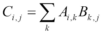
The following example shows the Hadamard product and dot product using tensor objects:

import tensorflow as tf

mat1 = tf.constant([[4, 5, 6],[3,2,1]])
mat2 = tf.constant([[7, 8, 9],[10, 11, 12]])

# hadamard product (element wise)
mult = tf.multiply(mat1, mat2)

# dot product (no. of rows = no. of columns)
dotprod = tf.matmul(mat1, tf.transpose(mat2))

with tf.Session() as sess:
    print(sess.run(mult))
    print(sess.run(dotprod))

The output of the listing is shown as follows:

[[28 40 54][30 22 12]]
 [[122 167][ 46 64]]

Trace operator

The trace operator Tr(A) of matrix A gives the sum of all of the diagonal entries of a matrix. The following example shows how to use a trace operator on tensor objects:

import tensorflow as tf

mat = tf.constant([
 [0, 1, 2],
 [3, 4, 5],
 [6, 7, 8]
], dtype=tf.float32)

# get trace ('sum of diagonal elements') of the matrix
mat = tf.trace(mat)

with tf.Session() as sess:
    print(sess.run(mat))

The output of the listing is 12.0.

Matrix transpose

Transposition of the matrix is the mirror image of the matrix across the main diagonal. A symmetric matrix is any matrix that is equal to its own transpose:

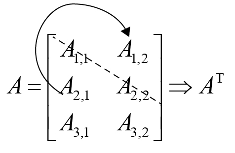
The following example shows how to use a transpose operator on tensor objects:

import tensorflow as tf

x = [[1,2,3],[4,5,6]]
x = tf.convert_to_tensor(x)
xtrans = tf.transpose(x)

y=([[[1,2,3],[6,5,4]],[[4,5,6],[3,6,3]]])
y = tf.convert_to_tensor(y)
ytrans = tf.transpose(y, perm=[0, 2, 1])

with tf.Session() as sess:
   print(sess.run(xtrans))
   print(sess.run(ytrans))

The output of the listing is shown as follows:

[[1 4] [2 5] [3 6]]

Matrix diagonals

Matrices that are diagonal in nature consist mostly of zeros and have non-zero entries only along the main diagonal. Not all diagonal matrices need to be square.

Using the diagonal part operation, we can get the diagonal of a given matrix, and to create a matrix with a given diagonal, we use the diag operation from tensorflow. The following example shows how to use diagonal operators on tensor objects:

import tensorflow as tf

mat = tf.constant([
 [0, 1, 2],
 [3, 4, 5],
 [6, 7, 8]
], dtype=tf.float32)

# get diagonal of the matrix
diag_mat = tf.diag_part(mat)

# create matrix with given diagonal
mat = tf.diag([1,2,3,4])

with tf.Session() as sess:
   print(sess.run(diag_mat))
   print(sess.run(mat))

The output of this is shown as follows:

[ 0.  4.  8.]
[[1 0 0 0][0 2 0 0] [0 0 3 0] [0 0 0 4]]

Identity matrix

An identity matrix is a matrix I that does not change any vector, like V, when multiplied by I.

The following example shows how to get the identity matrix for a given size:

import tensorflow as tf

identity = tf.eye(3, 3)

with tf.Session() as sess:
   print(sess.run(identity))  

The output of this is shown as follows:

[[ 1.  0.  0.] [ 0.  1.  0.] [ 0.  0.  1.]]

Inverse matrix

The matrix inverse of I is denoted as

. Consider the following equation; to solve it using inverse and different values of b, there can be multiple solutions for x. Note the property:

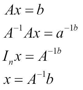
The following example shows how to calculate the inverse of a matrix using the matrix_inverse operation:

import tensorflow as tf

mat = tf.constant([[2, 3, 4], [5, 6, 7], [8, 9, 10]], dtype=tf.float32)
print(mat)

inv_mat = tf.matrix_inverse(tf.transpose(mat))

with tf.Session() as sess:
print(sess.run(inv_mat))

Solving linear equations

TensorFlow can solve a series of linear equations using the solve operation. Let's first explain this without using the library and later use the solve function.

A linear equation is represented as follows:

ax + b = yy - ax = b

y - ax = b

y/b - a/b(x) = 1

Our job is to find the values for a and b in the preceding equation, given our observed points. First, create the matrix points. The first column represents x values, while the second column represents y values. Consider that X is the input matrix and A is the parameters that we need to learn; we set up a system like AX=B, therefore,

. The following example, with code, shows how to solve the linear equation:

3x+2y = 154x−y = 10

import tensorflow as tf

# equation 1
x1 = tf.constant(3, dtype=tf.float32)
y1 = tf.constant(2, dtype=tf.float32)
point1 = tf.stack([x1, y1])

# equation 2
x2 = tf.constant(4, dtype=tf.float32)
y2 = tf.constant(-1, dtype=tf.float32)
point2 = tf.stack([x2, y2])

# solve for AX=C
X = tf.transpose(tf.stack([point1, point2]))
C = tf.ones((1,2), dtype=tf.float32)

A = tf.matmul(C, tf.matrix_inverse(X))

with tf.Session() as sess:
    X = sess.run(X)
    print(X)

    A = sess.run(A)
    print(A)

b = 1 / A[0][1]
a = -b * A[0][0]
print("Hence Linear Equation is: y = {a}x + {b}".format(a=a, b=b))

The output of the listing is shown as follows:

[[ 3. 4.][ 2. -1.]]
 [[ 0.27272728 0.09090909]]
Hence Linear Equation is: y = -2.9999999999999996x + 10.999999672174463

The canonical equation for a circle is x2+y2+dx+ey+f=0; to solve this for the parameters d, e, and f, we use TensorFlow's solve operation as follows:

# canonical circle equation
# x2+y2+dx+ey+f = 0
# dx+ey+f=−(x2+y2) ==> AX = B
# we have to solve for d, e, f

points = tf.constant([[2,1], [0,5], [-1,2]], dtype=tf.float64)
X = tf.constant([[2,1,1], [0,5,1], [-1,2,1]], dtype=tf.float64)
B = -tf.constant([[5], [25], [5]], dtype=tf.float64)

A = tf.matrix_solve(X,B)

with tf.Session() as sess:
    result = sess.run(A)
    D, E, F = result.flatten()
    print("Hence Circle Equation is: x**2 + y**2 + {D}x + {E}y + {F} = 0".format(**locals()))

The output of the listing is shown in the following code:

Hence Circle Equation is: x**2 + y**2 + -2.0x + -6.0y + 5.0 = 0

Singular value decomposition

When we decompose an integer into its prime factors, we can understand useful properties about the integer. Similarly, when we decompose a matrix, we can understand many functional properties that are not directly evident. There are two types of decomposition, namely eigenvalue decomposition and singular value decomposition.

All real matrices have singular value decomposition, but the same is not true for Eigenvalue decomposition. For example, if a matrix is not square, the Eigen decomposition is not defined and we must use singular value decomposition instead.

Singular Value Decomposition (SVD) in mathematical form is the product of three matrices U, S, and V, where U is m*r, S is r*r and V is r*n:

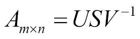
The following example shows SVD using a TensorFlow svd operation on textual data:

import numpy as np
import tensorflow as tf
import matplotlib.pyplot as plts

path = "/neuralnetwork-programming/ch01/plots"

text = ["I", "like", "enjoy",
         "deep", "learning", "NLP", "flying", "."]
xMatrix = np.array([[0,2,1,0,0,0,0,0],
              [2,0,0,1,0,1,0,0],
              [1,0,0,0,0,0,1,0],
              [0,1,0,0,1,0,0,0],
              [0,0,0,1,0,0,0,1],
              [0,1,0,0,0,0,0,1],
              [0,0,1,0,0,0,0,1],
              [0,0,0,0,1,1,1,0]], dtype=np.float32)

X_tensor = tf.convert_to_tensor(xMatrix, dtype=tf.float32)

# tensorflow svd
with tf.Session() as sess:
    s, U, Vh = sess.run(tf.svd(X_tensor, full_matrices=False))

for i in range(len(text)):
    plts.text(U[i,0], U[i,1], text[i])

plts.ylim(-0.8,0.8)
plts.xlim(-0.8,2.0)
plts.savefig(path + '/svd_tf.png')

# numpy svd
la = np.linalg
U, s, Vh = la.svd(xMatrix, full_matrices=False)

print(U)
print(s)
print(Vh)

# write matrices to file (understand concepts)
file = open(path + "/matx.txt", 'w')
file.write(str(U))
file.write("\n")
file.write("=============")
file.write("\n")
file.write(str(s))
file.close()

for i in range(len(text)):
    plts.text(U[i,0], U[i,1], text[i])

plts.ylim(-0.8,0.8)
plts.xlim(-0.8,2.0)
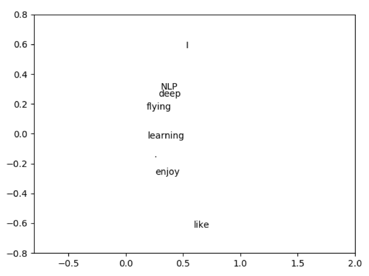
plts.savefig(path + '/svd_np.png')

The output of this is shown as follows:

[[ -5.24124920e-01  -5.72859168e-01   9.54463035e-02   3.83228481e-01   -1.76963374e-01  -1.76092178e-01  -4.19185609e-01  -5.57702743e-02]
[ -5.94438076e-01   6.30120635e-01  -1.70207784e-01   3.10038358e-0
 1.84062332e-01  -2.34777853e-01   1.29535481e-01   1.36813134e-01]
[ -2.56274015e-01   2.74017543e-01   1.59810841e-01   3.73903001e-16
  -5.78984618e-01   6.36550903e-01  -3.32297325e-16  -3.05414885e-01]
[ -2.85637408e-01  -2.47912124e-01   3.54610324e-01  -7.31901303e-02
  4.45784479e-01   8.36141407e-02   5.48721075e-01  -4.68012422e-01]
[ -1.93139315e-01   3.38495038e-02  -5.00790417e-01  -4.28462476e-01
 3.47110212e-01   1.55483231e-01  -4.68663752e-01  -4.03576553e-01]
[ -3.05134684e-01  -2.93989003e-01  -2.23433599e-01  -1.91614240e-01
 1.27460942e-01   4.91219401e-01   2.09592804e-01   6.57535374e-01]
[ -1.82489842e-01  -1.61027774e-01  -3.97842437e-01  -3.83228481e-01
 -5.12923241e-01  -4.27574426e-01   4.19185609e-01  -1.18313827e-01]
[ -2.46898428e-01   1.57254755e-01   5.92991650e-01  -6.20076716e-01
 -3.21868137e-02  -2.31065080e-01  -2.59070963e-01   2.37976909e-01]]
[ 2.75726271  2.67824793  1.89221275  1.61803401  1.19154561  0.94833982
 0.61803401  0.56999218]
[[ -5.24124920e-01  -5.94438076e-01  -2.56274015e-01  -2.85637408e-01
 -1.93139315e-01  -3.05134684e-01  -1.82489842e-01  -2.46898428e-01]
[  5.72859168e-01  -6.30120635e-01  -2.74017543e-01   2.47912124e-01
 -3.38495038e-02   2.93989003e-01   1.61027774e-01  -1.57254755e-01]
[ -9.54463035e-02   1.70207784e-01  -1.59810841e-01  -3.54610324e-01
 5.00790417e-01   2.23433599e-01   3.97842437e-01  -5.92991650e-01]
[  3.83228481e-01   3.10038358e-01  -2.22044605e-16  -7.31901303e-02
 -4.28462476e-01  -1.91614240e-01  -3.83228481e-01  -6.20076716e-01]
[ -1.76963374e-01   1.84062332e-01  -5.78984618e-01   4.45784479e-01
 3.47110212e-01   1.27460942e-01  -5.12923241e-01  -3.21868137e-02]
[  1.76092178e-01   2.34777853e-01  -6.36550903e-01  -8.36141407e-02
 -1.55483231e-01  -4.91219401e-01   4.27574426e-01   2.31065080e-01]
[  4.19185609e-01  -1.29535481e-01  -3.33066907e-16  -5.48721075e-01
  4.68663752e-01  -2.09592804e-01  -4.19185609e-01   2.59070963e-01]
[ -5.57702743e-02   1.36813134e-01  -3.05414885e-01  -4.68012422e-01
 -4.03576553e-01   6.57535374e-01  -1.18313827e-01   2.37976909e-01]]

Here is the plot for the SVD of the preceding dataset:

Eigenvalue decomposition

Eigen decomposition is one of the most famous decomposition techniques in which we decompose a matrix into a set of eigenvectors and eigenvalues.

For a square matrix, Eigenvector is a vector v such that multiplication by A alters only the scale of v:

Av = λv

The scalar λ is known as the eigenvalue corresponding to this eigenvector.

Eigen decomposition of A is then given as follows:

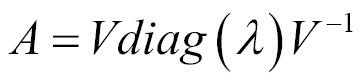
Eigen decomposition of a matrix describes many useful details about the matrix. For example, the matrix is singular if, and only if, any of the eigenvalues are zero.

Principal Component Analysis

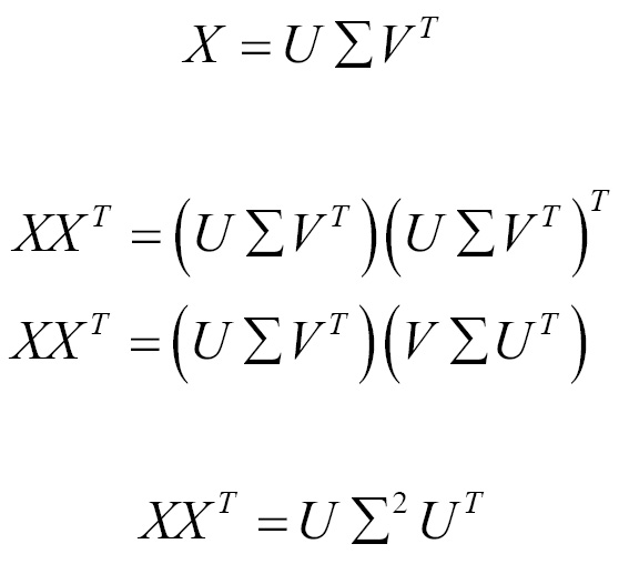
Principal Component Analysis (PCA) projects the given dataset onto a lower dimensional linear space so that the variance of the projected data is maximized. PCA requires the eigenvalues and eigenvectors of the covariance matrix, which is the product where X is the data matrix.

SVD on the data matrix X is given as follows:

The following example shows PCA using SVD:

import numpy as np
import tensorflow as tf
import matplotlib.pyplot as plt
import plotly.plotly as py
import plotly.graph_objs as go
import plotly.figure_factory as FF
import pandas as pd

path = "/neuralnetwork-programming/ch01/plots"
logs = "/neuralnetwork-programming/ch01/logs"

xMatrix = np.array([[0,2,1,0,0,0,0,0],
              [2,0,0,1,0,1,0,0],
              [1,0,0,0,0,0,1,0],
              [0,1,0,0,1,0,0,0],
              [0,0,0,1,0,0,0,1],
              [0,1,0,0,0,0,0,1],
              [0,0,1,0,0,0,0,1],
              [0,0,0,0,1,1,1,0]], dtype=np.float32)

def pca(mat):
    mat = tf.constant(mat, dtype=tf.float32)
    mean = tf.reduce_mean(mat, 0)
    less = mat - mean
    s, u, v = tf.svd(less, full_matrices=True, compute_uv=True)

    s2 = s ** 2
    variance_ratio = s2 / tf.reduce_sum(s2)

    with tf.Session() as session:
        run = session.run([variance_ratio])
    return run


if __name__ == '__main__':
    print(pca(xMatrix))

The output of the listing is shown as follows:

[array([  4.15949494e-01,   2.08390564e-01,   1.90929279e-01,
         8.36438537e-02,   5.55494241e-02,   2.46047471e-02,
         2.09326427e-02,   3.57540098e-16], dtype=float32)]