Calculus

Topics in the previous sections are covered as part of standard linear algebra; something that wasn't covered is basic calculus. Despite the fact that the calculus that we use is relatively simple, the mathematical form of it may look very complex. In this section, we present some basic forms of matrix calculus with a few examples.

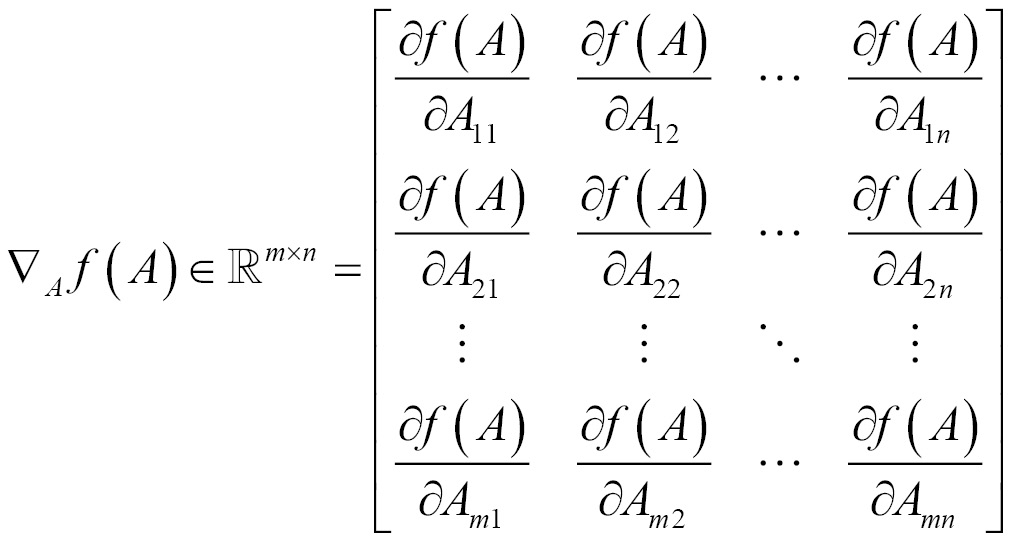
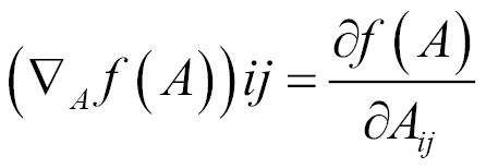
Gradient

Gradient for functions with respect to a real-valued matrixA is defined as the matrix of partial derivatives of A and is denoted as follows:

TensorFlow does not do numerical differentiation; rather, it supports automatic differentiation. By specifying operations in a TensorFlow graph, it can automatically run the chain rule through the graph and, as it knows the derivatives of each operation we specify, it can combine them automatically.

The following example shows training a network using MNIST data, the MNIST database consists of handwritten digits. It has a training set of 60,000 examples and a test set of 10,000 samples. The digits are size-normalized.

Here backpropagation is performed without any API usage and derivatives are calculated manually. We get 913 correct out of 1,000 tests. This concept will be introduced in the next chapter.

The following code snippet describes how to get the mnist dataset and initialize weights and biases:

import tensorflow as tf

# get mnist dataset
from tensorflow.examples.tutorials.mnist import input_data
data = input_data.read_data_sets("MNIST_data/", one_hot=True)

# x represents image with 784 values as columns (28*28), y represents output digit
x = tf.placeholder(tf.float32, [None, 784])
y = tf.placeholder(tf.float32, [None, 10])

# initialize weights and biases [w1,b1][w2,b2]
numNeuronsInDeepLayer = 30
w1 = tf.Variable(tf.truncated_normal([784, numNeuronsInDeepLayer]))
b1 = tf.Variable(tf.truncated_normal([1, numNeuronsInDeepLayer]))
w2 = tf.Variable(tf.truncated_normal([numNeuronsInDeepLayer, 10]))
b2 = tf.Variable(tf.truncated_normal([1, 10]))

We now define a two-layered network with a nonlinear sigmoid function; a squared loss function is applied and optimized using a backward propagation algorithm, as shown in the following snippet:

# non-linear sigmoid function at each neuron
def sigmoid(x):
    sigma = tf.div(tf.constant(1.0), tf.add(tf.constant(1.0), tf.exp(tf.negative(x))))
    return sigma

# starting from first layer with wx+b, then apply sigmoid to add non-linearity
z1 = tf.add(tf.matmul(x, w1), b1)
a1 = sigmoid(z1)
z2 = tf.add(tf.matmul(a1, w2), b2)
a2 = sigmoid(z2)

# calculate the loss (delta)
loss = tf.subtract(a2, y)

# derivative of the sigmoid function der(sigmoid)=sigmoid*(1-sigmoid)
def sigmaprime(x):
    return tf.multiply(sigmoid(x), tf.subtract(tf.constant(1.0), sigmoid(x)))

# backward propagation
dz2 = tf.multiply(loss, sigmaprime(z2))
db2 = dz2
dw2 = tf.matmul(tf.transpose(a1), dz2)

da1 = tf.matmul(dz2, tf.transpose(w2))
dz1 = tf.multiply(da1, sigmaprime(z1))
db1 = dz1
dw1 = tf.matmul(tf.transpose(x), dz1)

# finally update the network
eta = tf.constant(0.5)
step = [
    tf.assign(w1,
              tf.subtract(w1, tf.multiply(eta, dw1)))
    , tf.assign(b1,
                tf.subtract(b1, tf.multiply(eta,
                                             tf.reduce_mean(db1, axis=[0]))))
    , tf.assign(w2,
                tf.subtract(w2, tf.multiply(eta, dw2)))
    , tf.assign(b2,
                tf.subtract(b2, tf.multiply(eta,
                                             tf.reduce_mean(db2, axis=[0]))))
]

acct_mat = tf.equal(tf.argmax(a2, 1), tf.argmax(y, 1))
acct_res = tf.reduce_sum(tf.cast(acct_mat, tf.float32))

sess = tf.InteractiveSession()
sess.run(tf.global_variables_initializer())

for i in range(10000):
    batch_xs, batch_ys = data.train.next_batch(10)
    sess.run(step, feed_dict={x: batch_xs,
                              y: batch_ys})
    if i % 1000 == 0:
        res = sess.run(acct_res, feed_dict=
        {x: data.test.images[:1000],
         y: data.test.labels[:1000]})
        print(res)

The output of this is shown as follows:

Extracting MNIST_data
125.0
814.0
870.0
874.0
889.0
897.0
906.0
903.0
922.0
913.0

Now, let's use automatic differentiation with TensorFlow. The following example demonstrates the use of GradientDescentOptimizer. We get 924 correct out of 1,000 tests.

import tensorflow as tf

# get mnist dataset
from tensorflow.examples.tutorials.mnist import input_data
data = input_data.read_data_sets("MNIST_data/", one_hot=True)

# x represents image with 784 values as columns (28*28), y represents output digit
x = tf.placeholder(tf.float32, [None, 784])
y = tf.placeholder(tf.float32, [None, 10])

# initialize weights and biases [w1,b1][w2,b2]
numNeuronsInDeepLayer = 30
w1 = tf.Variable(tf.truncated_normal([784, numNeuronsInDeepLayer]))
b1 = tf.Variable(tf.truncated_normal([1, numNeuronsInDeepLayer]))
w2 = tf.Variable(tf.truncated_normal([numNeuronsInDeepLayer, 10]))
b2 = tf.Variable(tf.truncated_normal([1, 10]))

# non-linear sigmoid function at each neuron
def sigmoid(x):
    sigma = tf.div(tf.constant(1.0), tf.add(tf.constant(1.0), tf.exp(tf.negative(x))))
    return sigma

# starting from first layer with wx+b, then apply sigmoid to add non-linearity
z1 = tf.add(tf.matmul(x, w1), b1)
a1 = sigmoid(z1)
z2 = tf.add(tf.matmul(a1, w2), b2)
a2 = sigmoid(z2)

# calculate the loss (delta)
loss = tf.subtract(a2, y)

# derivative of the sigmoid function der(sigmoid)=sigmoid*(1-sigmoid)
def sigmaprime(x):
    return tf.multiply(sigmoid(x), tf.subtract(tf.constant(1.0), sigmoid(x)))

# automatic differentiation
cost = tf.multiply(loss, loss)
step = tf.train.GradientDescentOptimizer(0.1).minimize(cost)

acct_mat = tf.equal(tf.argmax(a2, 1), tf.argmax(y, 1))
acct_res = tf.reduce_sum(tf.cast(acct_mat, tf.float32))

sess = tf.InteractiveSession()
sess.run(tf.global_variables_initializer())

for i in range(10000):
    batch_xs, batch_ys = data.train.next_batch(10)
    sess.run(step, feed_dict={x: batch_xs,
                              y: batch_ys})
    if i % 1000 == 0:
        res = sess.run(acct_res, feed_dict=
        {x: data.test.images[:1000],
         y: data.test.labels[:1000]})
        print(res)

The output of this is shown as follows:

96.0
 777.0
 862.0
 870.0
 889.0
 901.0
 911.0
 905.0
 914.0
 924.0

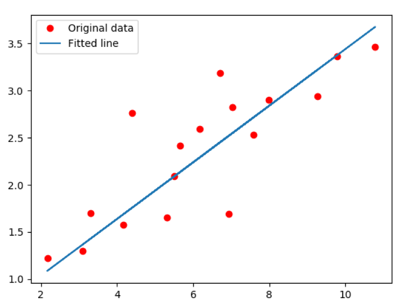
The following example shows linear regression using gradient descent:

import tensorflow as tf
import numpy
import matplotlib.pyplot as plt
rndm = numpy.random

# config parameters
learningRate = 0.01
trainingEpochs = 1000
displayStep = 50

# create the training data
trainX = numpy.asarray([3.3,4.4,5.5,6.71,6.93,4.168,9.779,6.182,7.59,2.167,
                         7.042,10.791,5.313,7.997,5.654,9.27,3.12])
trainY = numpy.asarray([1.7,2.76,2.09,3.19,1.694,1.573,3.366,2.596,2.53,1.221,
                         2.827,3.465,1.65,2.904,2.42,2.94,1.34])
nSamples = trainX.shape[0]

# tf inputs
X = tf.placeholder("float")
Y = tf.placeholder("float")

# initialize weights and bias
W = tf.Variable(rndm.randn(), name="weight")
b = tf.Variable(rndm.randn(), name="bias")

# linear model
linearModel = tf.add(tf.multiply(X, W), b)

# mean squared error
loss = tf.reduce_sum(tf.pow(linearModel-Y, 2))/(2*nSamples)

# Gradient descent
opt = tf.train.GradientDescentOptimizer(learningRate).minimize(loss)

# initializing variables
init = tf.global_variables_initializer()

# run
with tf.Session() as sess:
    sess.run(init)

    # fitting the training data
    for epoch in range(trainingEpochs):
        for (x, y) in zip(trainX, trainY):
            sess.run(opt, feed_dict={X: x, Y: y})

        # print logs
        if (epoch+1) % displayStep == 0:
            c = sess.run(loss, feed_dict={X: trainX, Y:trainY})
            print("Epoch is:", '%04d' % (epoch+1), "loss=", "{:.9f}".format(c), "W=", sess.run(W), "b=", sess.run(b))

    print("optimization done...")
    trainingLoss = sess.run(loss, feed_dict={X: trainX, Y: trainY})
    print("Training loss=", trainingLoss, "W=", sess.run(W), "b=", sess.run(b), '\n')

    # display the plot
    plt.plot(trainX, trainY, 'ro', label='Original data')
    plt.plot(trainX, sess.run(W) * trainX + sess.run(b), label='Fitted line')
    plt.legend()
    plt.show()

    # Testing example, as requested (Issue #2)
    testX = numpy.asarray([6.83, 4.668, 8.9, 7.91, 5.7, 8.7, 3.1, 2.1])
    testY = numpy.asarray([1.84, 2.273, 3.2, 2.831, 2.92, 3.24, 1.35, 1.03])

    print("Testing... (Mean square loss Comparison)")
    testing_cost = sess.run(
        tf.reduce_sum(tf.pow(linearModel - Y, 2)) / (2 * testX.shape[0]),
        feed_dict={X: testX, Y: testY})
    print("Testing cost=", testing_cost)
    print("Absolute mean square loss difference:", abs(trainingLoss - testing_cost))

    plt.plot(testX, testY, 'bo', label='Testing data')
    plt.plot(trainX, sess.run(W) * trainX + sess.run(b), label='Fitted line')
    plt.legend()
    plt.show()

The output of this is shown as follows:

Epoch is: 0050 loss= 0.141912043 W= 0.10565 b= 1.8382
 Epoch is: 0100 loss= 0.134377643 W= 0.11413 b= 1.7772
 Epoch is: 0150 loss= 0.127711013 W= 0.122106 b= 1.71982
 Epoch is: 0200 loss= 0.121811897 W= 0.129609 b= 1.66585
 Epoch is: 0250 loss= 0.116592340 W= 0.136666 b= 1.61508
 Epoch is: 0300 loss= 0.111973859 W= 0.143304 b= 1.56733
 Epoch is: 0350 loss= 0.107887231 W= 0.149547 b= 1.52241
 Epoch is: 0400 loss= 0.104270980 W= 0.15542 b= 1.48017
 Epoch is: 0450 loss= 0.101070963 W= 0.160945 b= 1.44043
 Epoch is: 0500 loss= 0.098239250 W= 0.166141 b= 1.40305
 Epoch is: 0550 loss= 0.095733419 W= 0.171029 b= 1.36789
 Epoch is: 0600 loss= 0.093516059 W= 0.175626 b= 1.33481
 Epoch is: 0650 loss= 0.091553882 W= 0.179951 b= 1.3037
 Epoch is: 0700 loss= 0.089817807 W= 0.184018 b= 1.27445
 Epoch is: 0750 loss= 0.088281371 W= 0.187843 b= 1.24692
 Epoch is: 0800 loss= 0.086921677 W= 0.191442 b= 1.22104
 Epoch is: 0850 loss= 0.085718453 W= 0.194827 b= 1.19669
 Epoch is: 0900 loss= 0.084653646 W= 0.198011 b= 1.17378
 Epoch is: 0950 loss= 0.083711281 W= 0.201005 b= 1.15224
 Epoch is: 1000 loss= 0.082877308 W= 0.203822 b= 1.13198
 optimization done...
 Training loss= 0.0828773 W= 0.203822 b= 1.13198
Testing... (Mean square loss Comparison)
 Testing cost= 0.0957726
 Absolute mean square loss difference: 0.0128952

The plots are as follows:

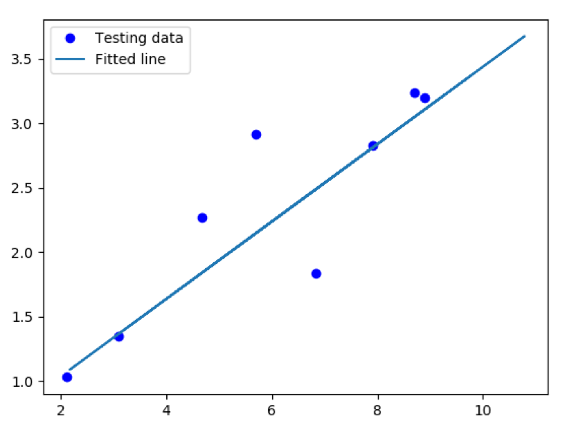
The following image shows the fitted line on testing data using the model:

Hessian

Gradient is the first derivative for functions of vectors, whereas hessian is the second derivative. We will go through the notation now:

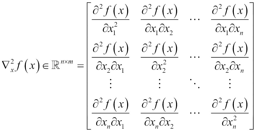
Similar to the gradient, the hessian is defined only when f(x) is real-valued.

Note

The algebraic function used is

.

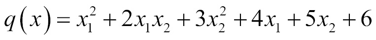
The following example shows the hessian implementation using TensorFlow:

import tensorflow as tf
import numpy as np

X = tf.Variable(np.random.random_sample(), dtype=tf.float32)
y = tf.Variable(np.random.random_sample(), dtype=tf.float32)

def createCons(x):
    return tf.constant(x, dtype=tf.float32)

function = tf.pow(X, createCons(2)) + createCons(2) * X * y + createCons(3) * tf.pow(y, createCons(2)) + createCons(4) * X + createCons(5) * y + createCons(6)

# compute hessian
def hessian(func, varbles):
    matrix = []
    for v_1 in varbles:
        tmp = []
        for v_2 in varbles:
            # calculate derivative twice, first w.r.t v2 and then w.r.t v1
            tmp.append(tf.gradients(tf.gradients(func, v_2)[0], v_1)[0])
        tmp = [createCons(0) if t == None else t for t in tmp]
        tmp = tf.stack(tmp)
        matrix.append(tmp)
    matrix = tf.stack(matrix)
    return matrix

hessian = hessian(function, [X, y])

sess = tf.Session()
sess.run(tf.initialize_all_variables())
print(sess.run(hessian))

The output of this is shown as follows:

 [[ 2.  2.] [ 2.  6.]]

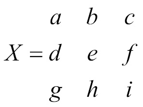
Determinant

Determinant shows us information about the matrix that is helpful in linear equations and also helps in finding the inverse of a matrix.

For a given matrix X, the determinant is shown as follows:

The following example shows how to get a determinant using TensorFlow:

import tensorflow as tf
import numpy as np

x = np.array([[10.0, 15.0, 20.0], [0.0, 1.0, 5.0], [3.0, 5.0, 7.0]], dtype=np.float32)

det = tf.matrix_determinant(x)

with tf.Session() as sess:
    print(sess.run(det))

The output of this is shown as follows:

-15.0