Creating the model
An Excel workbook can only contain one tabular model and that one model contains tables of data (which may or may not be related). The first step to create a model is to import data into it. There are many techniques to do this—some techniques have advantages over others but for now, let's only consider the fact that we want to load data that exists in an Excel worksheet into the model.
Tip
The installation instructions for PowerPivot in Excel 2010 are covered in the Appendix, Installing PowerPivot and Sample Databases, of this book.
Getting ready
Open the Excel workbook named SalesBook which is available from the Packt Publishing website to examine the worksheets within the book. Each sheet contains a dataset for Products, Subcategories, Categories, Customers, Dates, and Sales.
How to do it…
This recipe looks at importing data into the PowerPivot model through linked tables. These are very convenient to use when the data is stored in Excel. Additionally, once the data has been imported into PowerPivot, it retains a connection to the Excel table. This means that, when the data is changed in Excel, it can also be changed in the PowerPivot model.
- Let's start by importing the product list. Select the Product List sheet and select cell A1.
- Then, on the PowerPivot tab, click on the Create Linked Table button.
Tip
Excel will automatically highlight the data range.

- A small window will open confirming the data range with a checkbox for table headers. Select the checkbox and press OK.
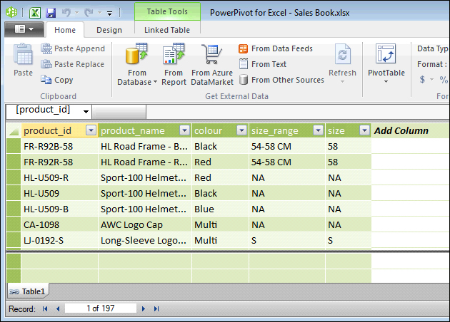
- The PowerPivot window will open and the data from the Product List sheet will be imported. Note that the table appears as a tab which is similar to Excel and is called Table1. Also, note that the PowerPivot window is a separate window than the Excel workbook, so that we can return to Excel.

- Repeat this process for all the remaining datasets except
Customers.
How it works…
When a linked table is created in PowerPivot, Excel creates a named range in the Excel workbook. This is then linked to the PowerPivot model (note that there is a small chain symbol before each of the tables). Also, note that the tables in Excel are formatted with alternate blue coloring. The named ranges can be viewed in Excel by clicking on the Name Manager button on the Formulas tab.

There's more…
A table (table range) is actually an Excel feature that PowerPivot utilizes. A table can be defined in Excel, given a meaningful name and then imported into PowerPivot, so that the name of the table in PowerPivot is the same as the named range in Excel.
Ensure that the Customers sheet is selected in Excel and also any cell in the Customers data is selected. In the Home tab, click on the Format as Table button, and choose a table style; the style chosen in the following screenshot is a relevant one:

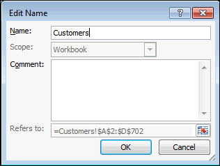
Note that the data is now formatted with alternating colors (based on the selected style). Return to the Name Manager window and double-click the table that relates to the Customers worksheet. A new window will open allowing you to edit the name, replace the name Table6 with Customers, and click on OK. The Table6 name is replaced by Customers in the Name Manager window.

Now, create a linked table in the same manner as we did before and note that the name of the table imported into PowerPivot is Customers.
Tip
If you want to select an entire table in Excel, simply choose the table name from the Name Box drop-down list in the formula bar in the upper-left corner. This is shown in the following screenshot:


