


Grasping the idea behind ML
The terms artificial intelligence (AI) and—partially—ML are omnipresent in today's world. However, a lot of what is found under the term AI is often nothing more than a containerized ML solution, and to make matters worse, ML is sometimes unnecessarily used to solve something extremely simple.
Therefore, in this first section, let's understand the class of problems ML tries to solve, in which scenarios to use ML, and when not to use it.
Problems and scenarios requiring ML
If you look for a definition of ML, you will often find a description such as this: It is the study of self-improving machine algorithms using data. ML is basically described as an algorithm we are trying to evolve, which in turn can be seen as one complex mathematical function.
Any computer process today follows the simple structure of the input-process-output (IPO) model. We define allowed inputs, we define a process working with those inputs, and we define an output through the type of results the process will show us. A simple example would be a word processing application, where every keystroke will result in a letter shown as the output on the screen. A completely different process might run in parallel to that one, having a time-based trigger to store the text file periodically to a hard disk.
All these processes or algorithms have one thing in common—they were manually written by someone using a high-level programming language. It is clear which actions need to be done when someone presses a letter in a word processing application. Therefore, we can easily build a process in which we implement which input values should create which output values.
Now, let's look at a more complex problem. Imagine we have a picture of a dog and want an application to just say: This is a dog. This sounds simple enough, as we know the input picture of a dog and the output value dog. Unfortunately, our brain (our own machine) is far superior to the machines we built, especially when it comes to pattern recognition. For a computer, a picture is just a square of  pixels, each containing three color channels defined by an 8-bit or 10-bit value. Therefore, an image is just a bunch of pixels made up of vectors for the computer, so in essence, a lot of numbers.
We could manually start writing an algorithm that maybe clusters groups of pixels, looks for edges and points of interest, and eventually, with a lot of effort, we might succeed in having an algorithm that finds dogs in pictures. That is when we get a picture of a cat.
It should be clear to you by now that we might run into a problem. Therefore, let's define one problem that ML solves, as follows:
Building the desired algorithm for a required solution programmatically is either extremely time-consuming, completely unfeasible, or impossible.
Taking this description, we can surely define good scenarios to use ML, be it finding objects in images and videos or understanding voices and extracting their intent from audio files. We will further understand what building ML solutions entails throughout this chapter (and the rest of the book, for that matter), but to make a simple statement, let's just acknowledge that building an ML model is also a time-consuming matter.
In that vein, it should be of utmost importance to avoid ML if we have the chance to do so. This might be an obvious statement, but as we (the authors) can attest, it is not for a lot of people. We have seen projects realized with ML where the output could be defined with a simple combination of if statements given some input vectors. In such scenarios, a solution could be obtained with a couple of hundred lines of code. Instead, months of training and testing an ML algorithm occurred, costing a lot of time and resources.
An example of this would be a company wanting to predict fraud (stolen money) committed by their own employees in a retail store. You might have heard that predicting fraud is a typical scenario for ML. Here, it was not necessary to use ML, as the company already knew the influencing factors (length of time the cashier was open, error codes on return receipts, and so on) and therefore wanted to be alerted when certain combinations of these factors occurred. As they knew the factors already, they could have just written the code and be done with it. But what does this scenario tell us about ML?
So far, we have looked at ML as a solution to solve a problem that, in essence, is too hard to code. Looking at the preceding scenario, you might understand another aspect or another class of problems that ML can solve. Therefore, let's add a second problem description, as follows:
Building the desired algorithm for a required solution is not feasible, as the influencing factors for the outcome of the desired outputs are only partially known or completely unknown.
Looking at this problem, you might now understand why ML relies so heavily on the field of statistics as, through the application of statistics, we can learn how data points influence one another, and therefore we might be able to solve such a problem. At the same time, we can build an algorithm that can find and predict the desired outcome.
In the previously mentioned scenario for detecting fraud, it might be prudent to still use ML, as it may be able to find a combination of influencing factors no one has thought about. But if this is not your set goal—as it was not in this case—you should not use ML for something that is easily written in code.
Now that we have discussed some of the problems solved by ML and have had a look at some scenarios for ML, let's have a look at how ML came to be.
The history of ML
To understand ML as a whole, we must first understand where it comes from. Therefore, let's delve into the history of ML. As with all events in history, different currents are happening simultaneously, adding pieces to the whole picture. We'll now look at a few important pillars that birthed the idea of ML as we know it today.
Learnings from neuroscience
A neuropsychologist named Donald O. Hebb published a book titled The Organization of Behavior in 1949. In this book, he described his theory of how neurons (neural cells) in our brain function, and how they contribute to what we understand as learning. This theory is known as Hebbian learning, and it makes the following proposition:
This basically describes that there is a process where one cell excites another repeatedly (the initiating cell) and maybe even the receiving cell is changed through a hidden process. This process is what we call learning.
To understand this a bit more visually, let's have a look at the biological structure of a neuron, as follows:
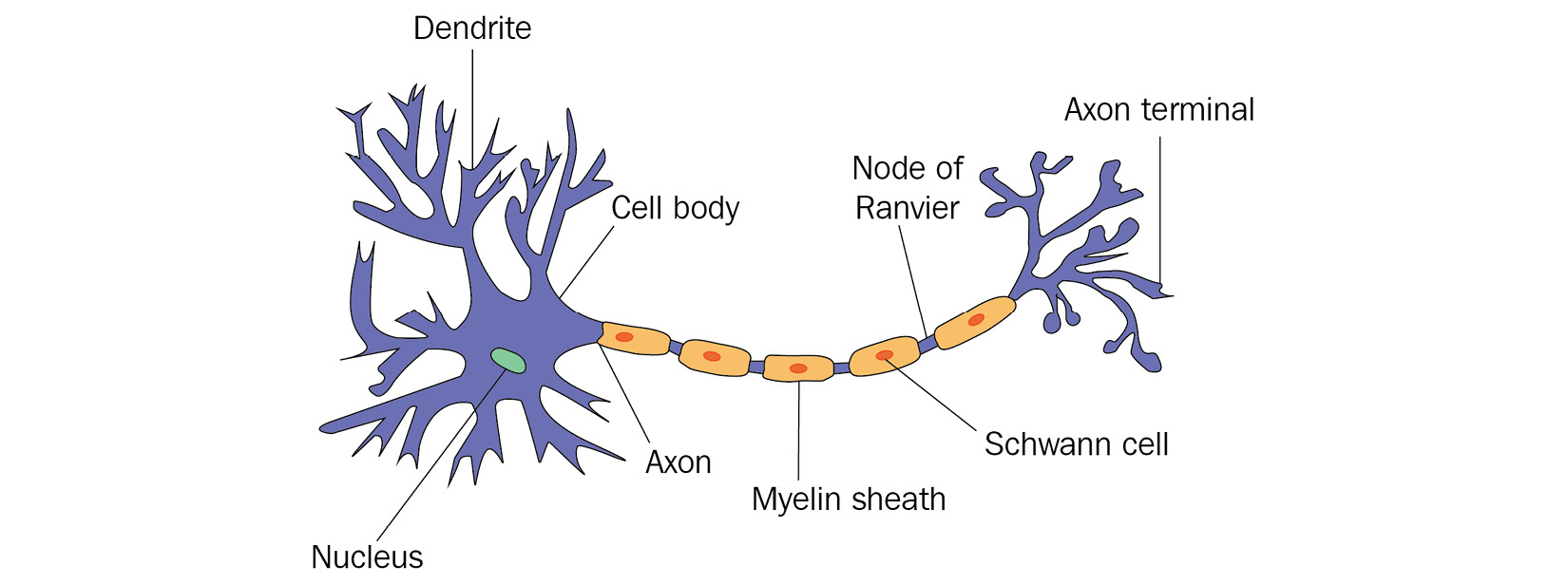
Figure 1.1 – Neuron in a biological neural network
What is visualized here? Firstly, on the left, we see the main body of the cell and its nucleus. The body receives input signals through dendrites that are connected to other neurons. In addition, there is a larger exit perturbing from the body called the axon, which connects the main body through a chain of Schwann cells to the so-called axon terminal, which in turn connects again to other neurons.
Looking at this structure with some creativity, it certainly resembles what a function or an algorithm might be. We have input signals coming from external neurons, we have some hidden process happening with these signals, and we have an output in the form of an axon terminal that connects the results to other neurons, and therefore other processes again.
It would take another decade again for someone to realize this connection.
Learnings from computer science
It is hard to talk about the history of ML in the context of computer science without mentioning one of the fathers of modern machines, Alan Turing. In a paper called Computing Machinery and Intelligence published in 1950, Turing defines a test called the Imitation Game (later called the Turing test) to evaluate whether a machine shows human behavior indistinguishable from a human. There are multiple iterations and variants of the test, but in essence, the idea is that a person would at no point in a conversation get the feeling they are not speaking with a human.
Certainly, this test is flawed, as there are ways to give relatively intelligent answers to questions while not being intelligent at all. If you want to learn more about this, have a look at ELIZA built by Joseph Weizenbaum, which passed the Turing test.
Nevertheless, this paper triggered one of the first discussions on what AI could be and what it means that a machine can learn.
Living in these exciting times, Arthur Samuel, a researcher working at International Business Machines Corporation (IBM) at that time, started developing a computer program that could make the right decisions in a game of checkers. In each move, he let the program evaluate a scoring function that tried to measure the chances of winning for each available move. Limited by the available resources at the time, it was not feasible to calculate all possible combinations of moves all the way to the end of the game.
This first step led to the definition of the so-called minimax algorithm and its accompanying search tree, which can commonly be used for any two-player adversarial game. Later, the alpha-beta pruning algorithm was added to automatically trim the tree from decisions that did not lead to better results than the ones already evaluated.
We are talking about Arthur Samuel, as it was he who coined the name machine learning, defining it as follows:
Combining these first ideas of building an evaluation function for training a machine and the research done by Donald O. Hebb in neuroscience, Frank Rosenblatt, a researcher at the Cornell Aeronautical Laboratory, invented a new linear classifier that he called a perceptron. Even though his progress in building this perceptron into hardware was relatively short-lived and would not live up to its potential, its original definition is nowadays the basis for every neuron in an artificial neural network (ANN).
Therefore, let's now dive deeper into understanding how ANNs work and what we can deduce about the inner workings of an ML algorithm from them.
Understanding the inner workings of ML through the example of ANNs
ANNs, as we know them today, are defined by the following two major components, one of which we learned about already:
- The neural network: The base structure of the system. A perceptron is basically an NN with only one neuron. By now, this structure comes in multiple facets, often involving hidden layers of hundreds of neurons, in the case of deep neural networks (DNNs).
- The backpropagation function: A rule for the system to learn and evolve. An idea thought of in the 1970s came into appreciation through a paper called Learning Representations by Back-Propagating Errors by D. Rumelhart, Geoffrey E. Hinton, Ronald J. Williams in 1986.
To understand these two components and how they work in tandem with each other, let's have a deeper look at both.
The neural network
First, let's understand how a single neuron operates, which is very close to the idea of a perceptron defined by Rosenblatt. The following diagram shows the inner workings of such an artificial neuron:
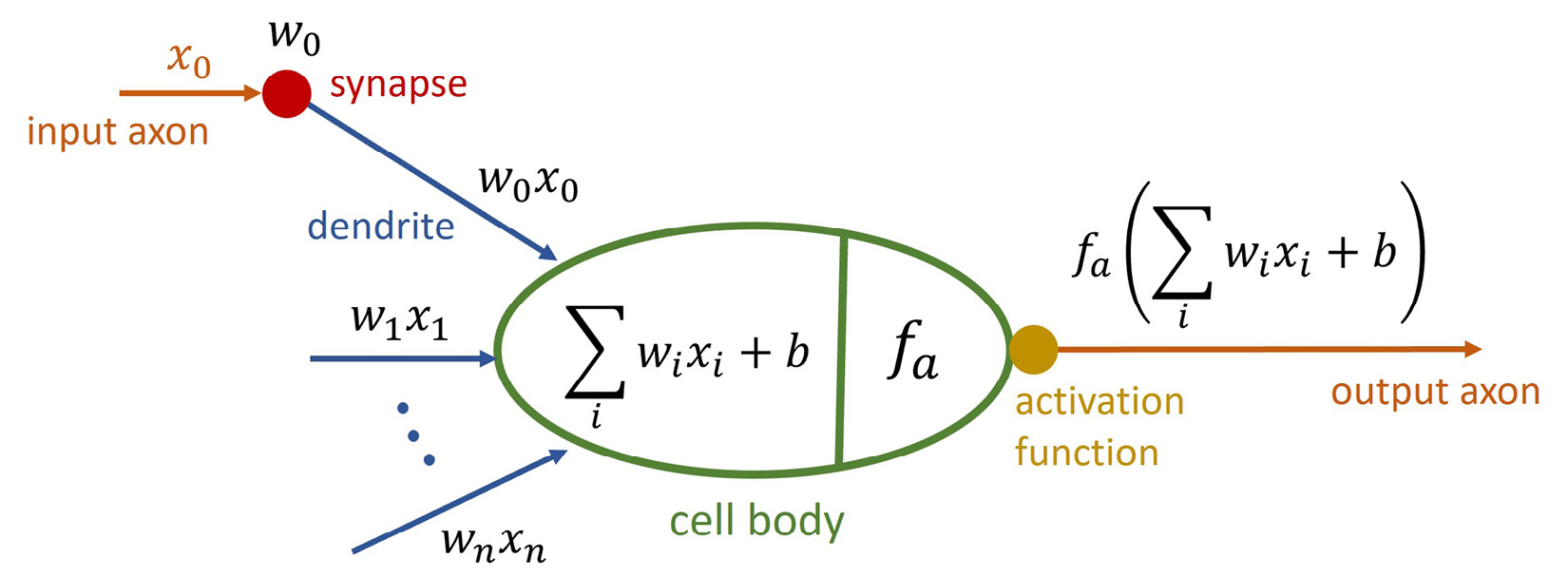
Figure 1.2 – Neuron in an ANN
We can clearly see the similarities to a real neuron. We get inputs from the connected neurons called  . Each of those inputs is weighted with a corresponding weight
  , and then, in the neuron itself, they are all summed up, including a bias
  . This is often referred to as the net input function.
As the final operation, a so-called activation function  is applied to this net input that decides how the output signal of the neuron should look. This function must be continuous and differentiable and should typically create results in the range of [0:1] or [-1:1] to keep results scaled. In addition, this function could be linear or non-linear in nature, even though using a linear activation function has its downfalls, as described next:
- You cannot learn a non-linear relationship presented in your data through a system of linear functions.
- A multilayered network made up of nodes with only linear activation functions can be broken down to just one layer of nodes with one linear activation function, making the network obsolete.
- You cannot use a linear activation function with backpropagation, as this requires calculating the derivative of this function, which we will discuss next.
Commonly used activation functions are sigmoid, hyperbolic tangent (tanh), rectified linear unit (ReLU), and softmax. Keeping this in mind, let's have a look at how we connect neurons together to achieve an ANN. A whole network is typically defined by three types of layers, as outlined here:
- Input layer: Consists of neurons accepting singular input signals (not a weighted sum) to the network. Their weights might be constant or randomized depending on the application.
- Hidden layer: Consists of the types of neurons we described before. They are defined by an activation function and given weights to the weighted sum of the input signals. In DNNs, these layers typically represent specific transformation steps.
- Output layer: Consists of neurons performing the final transformation of the data. They can behave like neurons in hidden layers, but they do not have to.
These together result in a typical ANN, as shown in the following diagram:
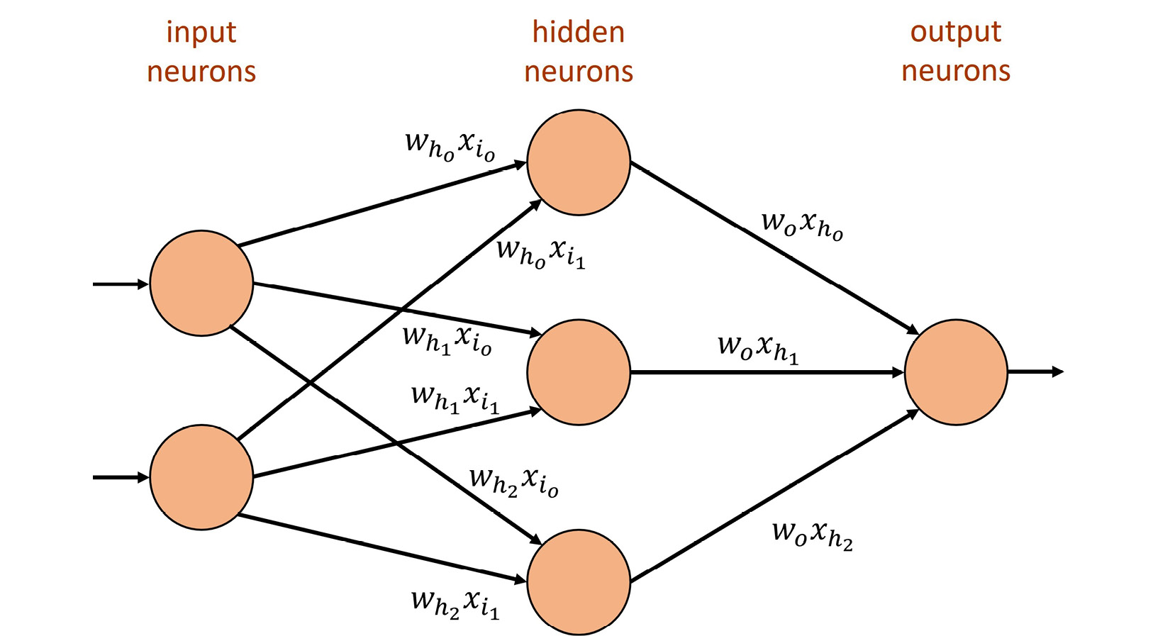
Figure 1.3 – ANN with one hidden layer
With this, we build a generic structure that can receive some input, realize some form of mathematical function through different layers of weights and activation functions, and in the end, hopefully show the correct output. This process of pushing information through the network from inputs to outputs is typically referred to as forward propagation. This, of course, only shows us what is happening with an input that passes through the network. The following question remains: How does it learn the desired function in the first place? The next section will answer this question.
The backpropagation function
The question that should have popped up in your mind by now is: How do we define the correct output? To have a way to change the behavior of the network, which mostly boils down to changing the values of the weights in the system, don't we need a way to quantize the error the system made?
Therefore, we need a function describing the error or loss, referred to as a loss function or error function. You might have even heard another name—a cost function. Let's define them next.
Loss Function versus Cost Function
A loss function (error function) computes the error for a single training example. A cost function, on the other hand, averages all loss function results for the entire training dataset.
This is the correct definition for those terms, but they are often used interchangeably. Just keep in mind that we are using some form of metric to measure the error we made or the distance we have from the correct results.
In classic backpropagation and other ML scenarios, the mean squared error (MSE) between the correct  and the computed
  is used to define the error or loss of the operation. The obvious target is to now minimize this error. Therefore, the actual task to perform is to find the total minimum of this function in n-dimensional space.
To do this, we use something that is often referred to as an optimizer, defined next.
Optimizer (Objective Function)
An optimizer is a function that implements a specific way to reach the objective of minimizing the cost function.
One such optimizer is an iterative process called gradient descent. Its idea is visualized in the following screenshot:
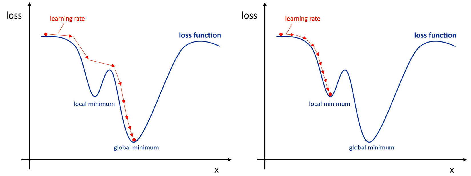
Figure 1.4 – Gradient descent with loss function influenced by only one input (left: finding global minimum, right: stuck in local minimum)
In gradient descent, we try to navigate an n-dimensional loss function by taking reasonably large enough steps, often defined by a learning rate, with the goal to find the global minimum, while avoiding getting stuck in a local minimum.
Keeping this in mind and without going into too much detail, let's finish this thought by going through the steps the backpropagation algorithm performs on the neural network. These are set out here:
- Pass a pair
 through the network (forward propagation).
 - Compute the loss between the expected
 and the computed
  .
. - Compute all derivatives for all functions and weights throughout the layers using a mathematical chain rule.
- Update all weights beginning from the back of the network to the front, with slightly changed weights defined by the optimizer.
- Repeat until convergence is achieved (the weights are not receiving any meaningful updates anymore).
This is, in a nutshell, how an ANN learns. Be aware that it is vital to constantly change the pairs in Step 1, as otherwise, you might push the network too far into memorizing these couple of pairs you constantly showed it. We will discuss the phenomenon of overfitting and underfitting later in this chapter.
As a final step in this section, let's now bring together what we have learned so far about ML and what this means for building software solutions in the future.
ML and Software 2.0
What we learned so far is that ML seems to be defined by a base structure with various knobs and levers (settings and values) that can be changed. In the case of ANNs, that would be the structure of the network itself and the weights, bias, and activation function we can set in some regard.
Accompanying this base structure is some sort of rule or function as to how these knobs and levers should be transformed through a learning process. In the case of ANNs, this is defined through the backpropagation function, which combines a loss function with an optimizer and some math.
In 2017, Andrej Karpathy, the chief technical officer (CTO) of Tesla's AI division, proposed that the aforementioned idea could be just another way of programming, which he called Software 2.0 (https://karpathy.medium.com/software-2-0-a64152b37c35).
Up to this point, writing software was about explaining to the machine precisely what it must do and what outcome it must produce through defining specific commands it had to follow. In this classical software development paradigm, we define algorithms by their code and let data run through it, typically written in a reasonably readable language.
Instead of doing that, another idea could be to define a program we build by a base structure, a way to evolve this structure, and the type of data it must process. In this case, we get something very human-unfriendly to understand (an ANN with weights, for example), but it might be much better to understand for a machine.
So, we leave you at the end of this section with the thought that Andrej wanted to convey. Perhaps ML is just another form of programming machines.
Keeping all this in mind, let's now talk about math.


