Probabilistic forecasting with DeepAR
This time, we’ll turn our attention to DeepAR, a state-of-the-art method for probabilistic forecasting. We’ll also leverage the neuralforecast framework to exemplify how to apply DeepAR for this task.
Getting ready
We’ll continue with the same dataset that we used in the previous recipe.
Since we are using a different Python package, we need to change our preprocessing steps to get the data into a suitable format. Now, each row corresponds to a single observation at a given time for a specific time series. This is similar to what we did in the Prediction intervals using conformal prediction recipe:
def load_and_prepare_data(file_path, time_column, series_column,
    aggregation_freq):
    """Load the time series data and prepare it for modeling."""
    dataset = pd.read_csv(file_path, parse_dates=[time_column])
    dataset.set_index(time_column, inplace=True)
    target_series = (
        dataset[series_column].resample(aggregation_freq).mean()
    )
    return target_series
def add_time_features(dataframe, date_column):
    """Add time-related features to the DataFrame."""
    dataframe["week_of_year"] = (
        dataframe[date_column].dt.isocalendar().week.astype(float)
    )
    dataframe["month"] = dataframe[date_column].dt.month.astype(float)
    dataframe["sin_week"] = np.sin(
        2 * np.pi * dataframe["week_of_year"] / 52
    )
    dataframe["cos_week"] = np.cos(
        2 * np.pi * dataframe["week_of_year"] / 52
    )
    dataframe["sin_2week"] = np.sin(
        4 * np.pi * dataframe["week_of_year"] / 52
    )
    dataframe["cos_2week"] = np.cos(
        4 * np.pi * dataframe["week_of_year"] / 52
    )
    dataframe["sin_month"] = np.sin(
        2 * np.pi * dataframe["month"] / 12
    )
    dataframe["cos_month"] = np.cos(
        2 * np.pi * dataframe["month"] / 12
    )
    return dataframe
def scale_features(dataframe, feature_columns):
    """Scale features."""
    scaler = MinMaxScaler()
    dataframe[feature_columns] = (
        scaler.fit_transform(dataframe[feature_columns])
    )
    return dataframe, scaler
FILE_PATH = "assets/daily_multivariate_timeseries.csv"
TIME_COLUMN = "datetime"
TARGET_COLUMN = "Incoming Solar"
AGGREGATION_FREQ = "W"
weekly_data = load_and_prepare_data(
    FILE_PATH, TIME_COLUMN, TARGET_COLUMN, AGGREGATION_FREQ
)
weekly_data = (
    weekly_data.reset_index().rename(columns={TARGET_COLUMN: "y"})
)
weekly_data = add_time_features(weekly_data, TIME_COLUMN)
numerical_features = [
    "y",
    "week_of_year",
    "sin_week",
    "cos_week",
    "sin_2week",
    "cos_2week",
    "sin_month",
    "cos_month",
]
features_to_scale = ["y", "week_of_year"]
weekly_data, scaler = scale_features(weekly_data, features_to_scale)
In this case, we select the targeted series within the dataset and resample it to a weekly frequency, aggregating the data points using the mean.
Next, we show how to enhance the dataset by adding time-related features. We introduce Fourier series components for the week and month of the year. By incorporating sine and cosine transformations, we capture the cyclical nature of time in our data. Additionally, we scale the target using a MinMaxScaler.
Finally, we split our dataset into training and testing sets:
def split_data(dataframe, date_column, split_time):
    """Split the data into training and test sets."""
    train = dataframe[dataframe[date_column] <= split_time]
    test = dataframe[dataframe[date_column] > split_time]
    return train, test
SPLIT_TIME = weekly_data["ds"].max() - pd.Timedelta(weeks=52)
train, test = split_data(weekly_data, "ds", SPLIT_TIME)
Now, let’s see how to build a DeepAR model using neuralforecast.
How to do it…
With the data prepared, we can define and train the DeepAR model. The NeuralForecast class receives a list of models as input. In this case, we only define the DeepAR class. The library provides a straightforward way to specify the architecture and training behavior of the model. After training, we generate forecasts using the predict() method:
nf = NeuralForecast(
    models=[
        DeepAR(
            h=52,
            input_size=52,
            lstm_n_layers=3,
            lstm_hidden_size=128,
            trajectory_samples=100,
            loss=DistributionLoss(
                distribution="Normal", level=[80, 90],
                    return_params=False
            ),
            futr_exog_list=[
                "week_of_year",
                "sin_week",
                "cos_week",
                "sin_2week",
                "cos_2week",
                "sin_month",
                "cos_month",
            ],
            learning_rate=0.001,
            max_steps=1000,
            val_check_steps=10,
            start_padding_enabled=True,
            early_stop_patience_steps=30,
            scaler_type="identity",
            enable_progress_bar=True,
        ),
    ],
    freq="W",
)
nf.fit(df=train, val_size=52)
Y_hat_df = nf.predict(
    futr_df=test[
        [
            "ds",
            "unique_id",
            "week_of_year",
            "sin_week",
            "cos_week",
            "sin_2week",
            "cos_2week",
            "sin_month",
            "cos_month",
        ]
    ]
)
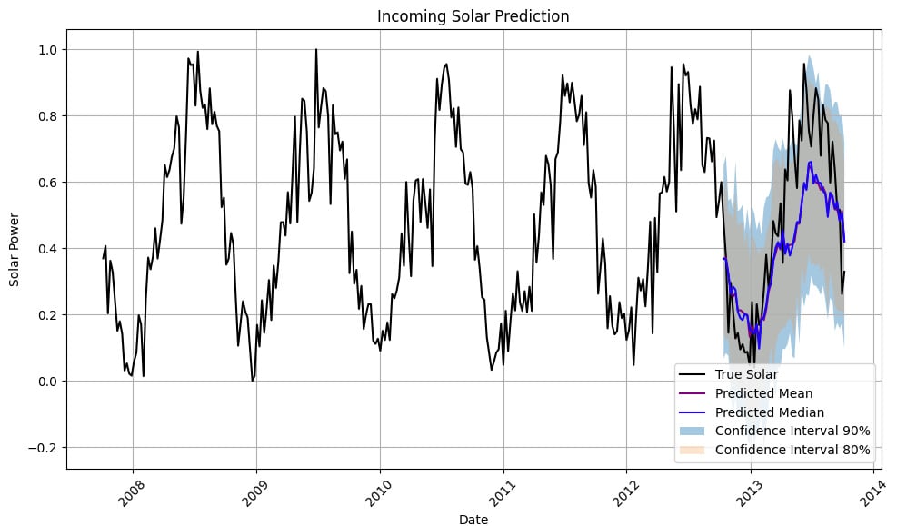
The following figure illustrates a probabilistic forecast generated by DeepAR:

Figure 7.6: DeepAR probabilistic forecast showing the mean prediction and associated uncertainty
The solid line represents the mean prediction, while the shaded region shows the uncertainty bounds for the 80% and 95% confidence intervals. This plot shows the range of likely future values and is more informative than a single predicted value, especially for decision-making under uncertainty.
How it works…
DeepAR is a probabilistic forecasting method that generates a probability distribution, such as a normal distribution or a negative binomial distribution, for each future time point. Once again, we are interested in capturing the uncertainty in our predictions rather than just producing point forecasts.
The DeepAR model uses an autoregressive recurrent network structure and conditions it on past observations, covariates, and an embedding of the time series. The output is a set of parameters, typically the mean and variance, which define the distribution of future values. During training, the model maximizes the likelihood of the observed data given these parameters.
DeepAR is designed to work well with multiple related time series, enabling it to learn complex patterns across similar sequences and improve prediction accuracy by leveraging cross-series information.


