Loading and visualizing a multivariate time series
So far, we’ve learned how to analyze univariate time series. Yet, multivariate time series are also relevant in real-world problems. This recipe explores how to load a multivariate time series. Before, we used the pandas Series structure to handle univariate time series. Multivariate time series are better structured as pandas DataFrame objects.
Getting ready
A multivariate time series contains multiple variables. The concepts underlying time series analysis are extended to cases where multiple variables evolve over time and are interrelated with each other. The relationship between the different variables can be difficult to model, especially when the number of these variables is large.
In many real-world applications, multiple variables can influence each other and exhibit a temporal dependency. For example, in weather modeling, the incoming solar radiation is correlated with other meteorological variables, such as air temperature or humidity. Considering these variables with a single multivariate model can be fundamental for modeling the dynamics of the data and getting better predictions.
We’ll continue to study the solar radiation dataset. This time series is extended by including extra meteorological information.
How to do it…
We’ll start by reading a multivariate time series. Like in the Loading a time series using pandas recipe, we resort to pandas and read a .csv file into a DataFrame data structure:
import pandas as pd
data = pd.read_csv('path/to/multivariate_ts.csv',
                   parse_dates=['datetime'],
                   index_col='datetime')
The parse_dates and index_col arguments ensure that the index of the DataFrame is a DatetimeIndex object. This is important so that pandas treats this object as a time series. After loading the time series, we can transform and visualize it using the plot() method:
data_log = LogTransformation.transform(data)
sample = data_log.tail(1000)
mv_plot = sample.plot(figsize=(15, 8),
                      title='Multivariate time series',
                      xlabel='',
                      ylabel='Value')
mv_plot.legend(fancybox=True, framealpha=1)
The preceding code follows these steps:
- First, we transform the data using the logarithm.
- We take the last 1,000 observations to make the visualization less cluttered.
- Finally, we use the
plot()method to create a visualization. We also calllegendto configure the legend of the plot.
How it works…
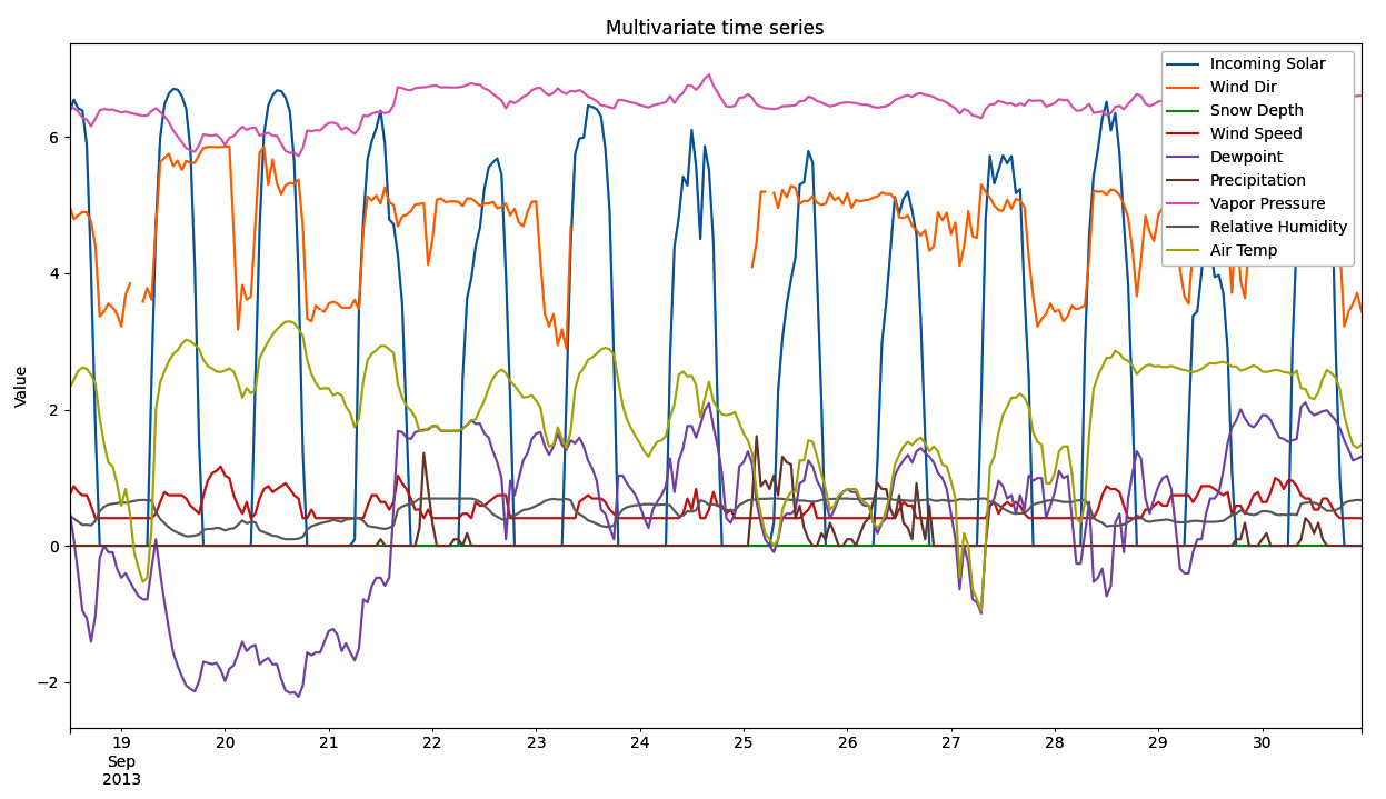
A sample of the multivariate time series is displayed in the following figure:

Figure 1.6: Multivariate time series plot
The process of loading a multivariate time series works like the univariate case. The main difference is that a multivariate time series is stored in Python as a DataFrame object rather than a Series one.
From the preceding plot, we can notice that different variables follow different distributions and have distinct average and dispersion levels.


