Search icon CANCEL
Subscription
0
Cart icon
Cart
Close icon
You have no products in your basket yet
Save more on your purchases!
Savings automatically calculated. No voucher code required
Arrow left icon
All Products
Best Sellers
New Releases
Books
Videos
Audiobooks
Learning Hub
Newsletters
Free Learning
Arrow right icon
Arrow up icon
GO TO TOP
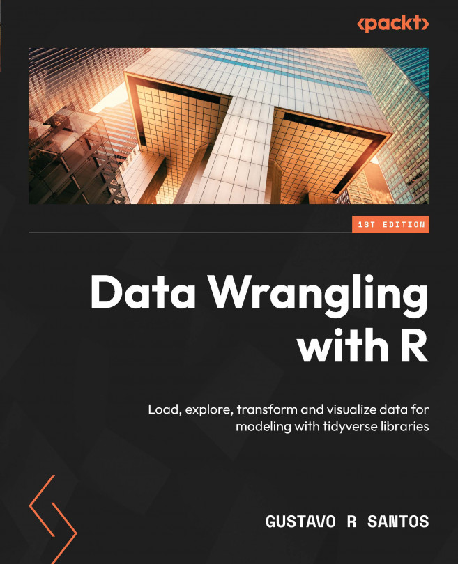
Data Wrangling with R

You're reading from  Data Wrangling with R

Product type Book
Published in Feb 2023
Publisher Packt
ISBN-13 9781803235400
Pages 384 pages
Edition 1st Edition
Languages
Concepts
Author (1):
Gustavo R Santos Gustavo R Santos
Profile icon Gustavo R Santos
Toc

Table of Contents (21) Chapters close

Preface 1. Part 1: Load and Explore Data
2. Chapter 1: Fundamentals of Data Wrangling 3. Chapter 2: Loading and Exploring Datasets 4. Chapter 3: Basic Data Visualization 5. Part 2: Data Wrangling
6. Chapter 4: Working with Strings 7. Chapter 5: Working with Numbers 8. Chapter 6: Working with Date and Time Objects 9. Chapter 7: Transformations with Base R 10. Chapter 8: Transformations with Tidyverse Libraries 11. Chapter 9: Exploratory Data Analysis 12. Part 3: Data Visualization
13. Chapter 10: Introduction to ggplot2 14. Chapter 11: Enhanced Visualizations with ggplot2 15. Chapter 12: Other Data Visualization Options 16. Part 4: Modeling
17. Chapter 13: Building a Model with R 18. Chapter 14: Build an Application with Shiny in R 19. Conclusion 20. Other Books You May Enjoy

Plot types

In Chapter 3, when studying basic data visualization, we used the mtcars toy dataset. In this chapter, we will go back to it, now being able to explore the capabilities of the ggplot2 library, as well as compare it to the base R plots previously created.

To load the dataset into an RStudio session and code along with this book, use the data("mtcars") code. To make the code more generic and transferable to other data frames, I will call the dataset df.

Histograms

Histograms are created using the geom_histogram() function. As usual, the same questions are applicable here to write the code:

  • What is the dataset? df.
  • What is the kind of graphic? Histogram.
  • What goes on x, and what is the color, fill color, and number of bins? Miles per gallon, with 20 bins.
  • What is the title of the plot? Histogram of Miles per Gallon:
# What is the dataset to be used?
ggplot(df) +
# What kind of graphic?
  geom_histogram( 
# What goes on...
lock icon The rest of the chapter is locked
Register for a free Packt account to unlock a world of extra content!
A free Packt account unlocks extra newsletters, articles, discounted offers, and much more. Start advancing your knowledge today.
Unlock this book and the full library FREE for 7 days
Get unlimited access to 7000+ expert-authored eBooks and videos courses covering every tech area you can think of
Renews at $15.99/month. Cancel anytime