The Polars LazyFrame
One of the unique features that makes Polars even faster and more efficient is its lazy API. The lazy API uses lazy evaluation, a technique that delays the evaluation of an expression until its value is needed. That means your query is only executed when it’s needed. This allows Polars to apply query optimizations because Polars can look at and execute multiple transformation steps at once by looking at the computation graph as a whole only when you tell it to do so. On the other hand, with eager evaluation (another evaluation strategy you’d use with DataFrame), you process data every time per expression. Essentially, lazy evaluation gives you more efficient ways to process your data.
You can access the Polars lazy API by using what we call LazyFrame. As explained earlier, LazyFrame allows for automatic query optimizations and larger-than-RAM processing.
LazyFrame is the proffered way of using Polars simply because it has more features and abilities to handle your data better. In this recipe, you’ll learn how to create a LazyFrame as well as how to use useful methods and functions associated with LazyFrame.
How to do it...
We’ll explore a LazyFrame by creating it first. Here are the steps:
- Create a LazyFrame from scratch:
data = {'name': ['Sarah', 'Mike', 'Bob', 'Ashley']}
lf = pl.LazyFrame(data)
type(lf)
The preceding code will return the following output:
>> polars.lazyframe.frame.LazyFrame
- Use the
.collect()method to instruct Polars to process data:lf.collect().head()
The preceding code will return the following output:

Figure 1.9 – LazyFrame output
- Create a LazyFrame from a
.csvfile using the.scan_csv()method:lf = pl.scan_csv('../data/titanic_dataset.csv') lf.head().collect()The preceding code will return the following output:

Figure 1.10 – The output of using .scan_csv()
- Convert a LazyFrame from a DataFrame with the
.lazy()method:df = pl.read_csv('../data/titanic_dataset.csv') df.lazy().head(3).collect()The preceding code will return the following output:

Figure 1.11 – Convert a DataFrame into a LazyFrame
- Show the schema and width of LazyFrame:
lf.collect_schema()
The preceding code will return the following output:
>> Schema([('PassengerId', Int64), ('Survived', Int64), ('Pclass', Int64), ('Name', String), ('Sex', String), ('Age', Float64), ('SibSp', Int64), ('Parch', Int64), ('Ticket', String), ('Fare', Float64), ('Cabin', String), ('Embarked', String)])
lf.collect_schema().len()
The preceding code will return the following output:
>> 12
How it works...
The structure of LazyFrame is the same as that of DataFrame, but LazyFrame doesn’t process your query until it’s told to do so using .collect(). You can use this to trigger the execution of the computation graph or query of a LazyFrame. This operation materializes a LazyFrame into a DataFrame.
Note
You should keep in mind that some operations that are available in DataFrame are not available in LazyFrame (such as .pivot()). These operations require Polars to know the whole structure of the data, which LazyFrame is not capable of handling. However, once you use .collect() to materialize a DataFrame, you’ll be able to use all the available DataFrame methods on it.
The way in which you create a LazyFrame is similar to the method for creating a DataFrame. After you have created a LazyFrame, and once it’s been materialized with .collect(), LazyFrame is converted to DataFrame. That’s why you can call .head() on it after calling .collect().
Note
You may be aware of the .fetch() method that was available until Polars version 0.20.31. While it was useful for debugging purposes, there were some gotchas that were confusing to users. Since Polars version 1.0.0, this method is deprecated. It’s still available as ._fetch() for development purposes.
You will notice that when you read a .csv file or any other file in LazyFrame, you use scan instead of read. This allows you to read files in lazy mode, whereby your column selections and filtering get pushed down to the scan level. You essentially read only the data necessary for the operations you’re performing in your code. You can see that that’s much more efficient than reading the whole dataset first and then filtering it down. Again, reading and writing files will be covered in the next chapter.
LazyFrame has similar attributes to DataFrame. However, you’ll need to access those via the .collect_schema() method. Note that the same method is also available in DataFrame.
Note
Since Polars version 1.0.0, you’ll get a performance warning when using LazyFrame attributes such as .schema, .width, .dtypes, and .columns. The .collect_schema() method replaces those methods. With recent improvements and changes made to the lazy engine, resolving the schema is no longer free and it can be relatively expensive. To solve this, the .collect_schema() method was added.
The good news is that it’s easy to go back and forth between LazyFrame and DataFrame with .lazy() and .collect(). This allows you to use LazyFrame where possible and convert to DataFrame if certain operations are not available in the lazy API or if you don’t need features such as automatic query optimization and larger-than-RAM processing for your use case.
There’s more...
One unique feature of LazyFrame is the ability to inspect the query plan of your code. You can use either the .show_graph() or the .explain() method. The .show_graph() method visualizes the query plan, whereas the .explain() method simply prints it out using .show_graph():
(
    lf
    .select(pl.col('Name', 'Age'))
    .show_graph()
)
The preceding code will return the following output:

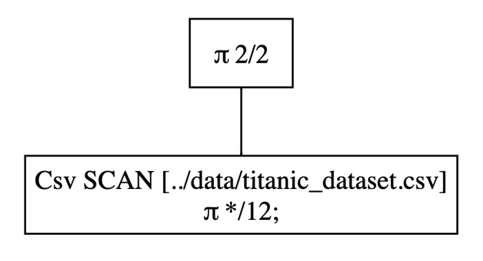
Figure 1.12 – A query execution plan
π (pi) indicates the column selection and σ (sigma) indicates the filtering conditions.
Note
I haven’t introduced the .filter() method yet, but just know that it’s used to filter data (it’s obvious, isn’t it?). We’ll cover it in a later recipe in this chapter: Selecting columns and filtering data.
By default, .show_graph() gives you the optimized query plan. You can customize its parameters to choose which optimization to apply. You can find more information on that here: https://pola-rs.github.io/polars/py-polars/html/reference/lazyframe/api/polars.LazyFrame.show_graph.html.
For now, here’s how to display the non-optimized version:
(
    lf
    .select(pl.col('Name', 'Age'))
    .show_graph(optimized=False)
)
The preceding code will return the following output:

Figure 1.13 – An optimized query execution plan
If you look carefully at both the optimized and the non-optimized version, you’ll notice that the former indicates two columns (π 2/12) whereas the latter indicates all columns (π */12).
Let’s try calling the .explain() method:
(
    lf
    .select(pl.col('Name', 'Age'))
    .explain()
)
The preceding code will return the following output:

Figure 1.14 – A query execution plan in text
You can tweak parameters with the .explain() method as well. You can find more information here: https://pola-rs.github.io/polars/py-polars/html/reference/lazyframe/api/polars.LazyFrame.explain.html.
The output of the .explain() method can be hard to read. To make it more readable, let’s try using Python’s built-in print() function with the separator specified:
print(
    lf
    .select(pl.col('Name', 'Age'))
    .explain()
    , sep='\n'
)
The preceding code will return the following output:

Figure 1.15 – A formatted query execution plan in text
We will dive more into inspecting and optimizing the query plan in Chapter 12, Testing and Debugging in Polars
See also
To learn more about LazyFrame, please visit these links:


