Demystifying neural networks

Here comes probably the most frequently mentioned model in the media, Artificial Neural Networks (ANNs); more often, we just call them neural networks. Interestingly, the neural network has been (falsely) considered equivalent to machine learning or artificial intelligence by the general public.

An ANN is just one type of algorithm among many in machine learning, and machine learning is a branch of artificial intelligence. It is one of the ways we achieve Artificial General Intelligence (AGI), which is a hypothetical type of AI that can think, learn, and solve problems like a human.

Regardless, it is one of the most important machine learning models and has been rapidly evolving along with the revolution of Deep Learning (DL).

Let’s first understand how neural networks work.

Starting with a single-layer neural network

We start by explaining different layers in a network, then move on to the activation function, and finally, training a network with backpropagation.

Layers in neural networks

A simple neural network is composed of three layers—the input layer, hidden layer, and output layer— as shown in the following diagram:

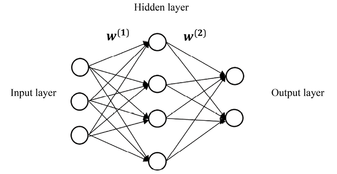
Figure 6.1: A simple shallow neural network

A layer is a conceptual collection of nodes (also called units), which simulate neurons in a biological brain. The input layer represents the input features, x, and each node is a predictive feature, x. The output layer represents the target variable(s).

In binary classification, the output layer contains only one node, whose value is the probability of the positive class. In multiclass classification, the output layer consists of n nodes, where n is the number of possible classes and the value of each node is the probability of predicting that class. In regression, the output layer contains only one node, the value of which is the prediction result.

The hidden layer can be considered a composition of latent information extracted from the previous layer. There can be more than one hidden layer. Learning with a neural network with two or more hidden layers is called deep learning. In this chapter, we will focus on one hidden layer to begin with.

Two adjacent layers are connected by conceptual edges (sort of like the synapses in a biological brain), which transmit signals from one neuron in a layer to another neuron in the next layer. The edges are parameterized by the weights, W, of the model. For example, W⁽¹⁾ in the preceding diagram connects the input and hidden layers and W⁽²⁾ connects the hidden and output layers.

In a standard neural network, data is conveyed only from the input layer to the output layer, through a hidden layer(s). Hence, this kind of network is called a feedforward neural network. Basically, logistic regression is a feedforward neural network with no hidden layer where the output layer connects directly with the input layer. Adding hidden layers between the input and output layers introduces non-linearity. This allows the neural networks to learn more about the underlying relationship between the input data and the target.

Activation functions

An activation function is a mathematical operation applied to the output of each neuron in a neural network. It determines whether the neuron should be activated (i.e., its output value should be propagated forward to the next layer) based on the input it receives.

Suppose the input, x, is of n dimensions, and the hidden layer is composed of H hidden units. The weight matrix, W⁽¹⁾, connecting the input and hidden layers is of size n by H, where each column, , represents the coefficients associating the input with the h-th hidden unit. The output (also called activation) of the hidden layer can be expressed mathematically as follows:

Here, f(z) is an activation function. As its name implies, the activation function checks how activated each neuron is, simulating the way our brains work. Their primary purpose is to introduce non-linearity into the output of a neuron, allowing the network to learn and perform complex mappings between inputs and outputs. Typical activation functions include the logistic function (more often called the sigmoid function in neural networks) and the tanh function, which is considered a rescaled version of the logistic function, as well as ReLU (short for Rectified Linear Unit), which is often used in DL:

We plot these three activation functions as follows:

• The logistic (sigmoid) function where the output value is in the range of (0, 1):

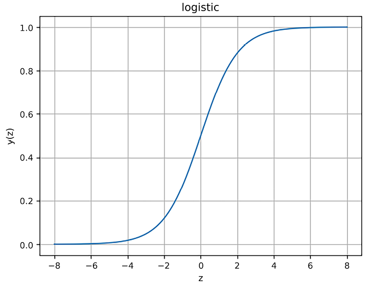
Figure 6.2: The logistic function

The visualization is produced by the following code:

>>> import numpy as np
>>> import matplotlib.pyplot as plt
>>> def sigmoid(z):
        return 1.0 / (1 + np.exp(-z))
>>> z = np.linspace(-8, 8, 1000)
>>> y = sigmoid(z)
>>> plt.plot(z, y)
>>> plt.xlabel('z')
>>> plt.ylabel('y(z)')
>>> plt.title('logistic')
>>> plt.grid()
>>> plt.show()

• The tanh function plot where the output value is in the range of (-1, 1):

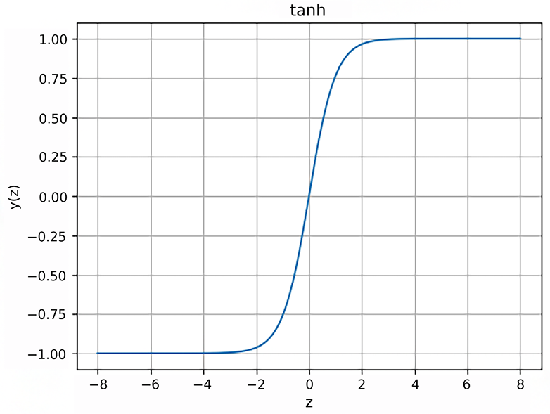
Figure 6.3: The tanh function

The visualization is produced by the following code:

>>> def tanh(z):
        return (np.exp(z) - np.exp(-z)) / (np.exp(z) + np.exp(-z))
>>> z = np.linspace(-8, 8, 1000)
>>> y = tanh(z)
>>> plt.plot(z, y)
>>> plt.xlabel('z')
>>> plt.ylabel('y(z)')
>>> plt.title('tanh')
>>> plt.grid()
>>> plt.show()

• The ReLU function plot where the output value is in the range of (0, +inf):

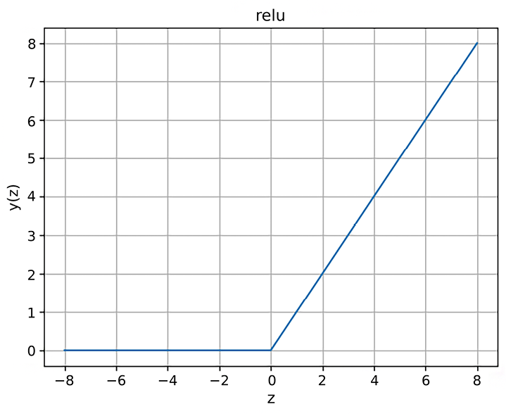
Figure 6.4: The ReLU function

The visualization is produced by the following code:

>>> relu(z):
        return np.maximum(np.zeros_like(z), z)
>>> z = np.linspace(-8, 8, 1000)
>>> y = relu(z)
>>> plt.plot(z, y)
>>> plt.xlabel('z')
>>> plt.ylabel('y(z)')
>>> plt.title('relu')
>>> plt.grid()
>>> plt.show()

As for the output layer, let’s assume that there is one output unit (regression or binary classification) and that the weight matrix, W⁽²⁾, connecting the hidden layer to the output layer is of size H by 1. In regression, the output can be expressed mathematically as follows (for consistency, I here denote it as a⁽³⁾ instead of y):

The Universal Approximation Theorem is a key concept in understanding how neural networks enable learning. It states that a feedforward neural network with a single hidden layer containing a finite number of neurons can approximate any continuous function to arbitrary precision, given a sufficiently large number of neurons in the hidden layer. During the training process, the neural network learns to approximate the target function by adjusting its parameters (weights). This is typically done using optimization algorithms, such as gradient descent, which iteratively update the parameters to minimize the difference between the predicted outputs and the true targets. Let’s see this process in detail in the next section.

Backpropagation

So, how can we obtain the optimal weights, W = {W(1), W(2)}, of the model? Similar to logistic regression, we can learn all weights using gradient descent with the goal of minimizing the mean squared error (MSE) cost or other loss function, J(W). The difference is that the gradients, , are computed through backpropagation. After each forward pass through a network, a backward pass is performed to adjust the model’s parameters.

As the word back in the name implies, the computation of the gradient proceeds backward: the gradient of the final layer is computed first and the gradient of the first layer is computed last. As for propagation, it means that partial computations of the gradient on one layer are reused in the computation of the gradient on the previous layer. Error information is propagated layer by layer, instead of being calculated separately.

In a single-layer network, the detailed steps of backpropagation are as follows:

1. We travel through the network from the input to the output and compute the output values, a⁽²⁾, of the hidden layer as well as the output layer, a⁽³⁾. This is the feedforward step.
2. For the last layer, we calculate the derivative of the cost function with regard to the input to the output layer:

3. For the hidden layer, we compute the derivative of the cost function with regard to the input to the hidden layer:

4. We compute the gradients by applying the chain rule:

1. We update the weights with the computed gradients and learning rate :

Here, m is the number of samples.

We repeatedly update all the weights by taking these steps with the latest weights until the cost function converges or the model goes through enough iterations.

The chain rule is a fundamental concept in calculus. It allows you to find the derivative of a composite function. You can read more in the mathematics course from Stanford University (https://mathematics.stanford.edu/events/chain-rule-calculus), or the differential calculus course, Module 6, Applications of Differentiation, from MIT (https://ocw.mit.edu/courses/18-03sc-differential-equations-fall-2011/).

This might not be easy to digest at first glance, so right after the next section, we will implement it from scratch, which will help you understand neural networks better.

Adding more layers to a neural network: DL

In real applications, a neural network usually comes with multiple hidden layers. That is how DL got its name—learning using neural networks with “stacked” hidden layers. An example of a DL model is as follows:

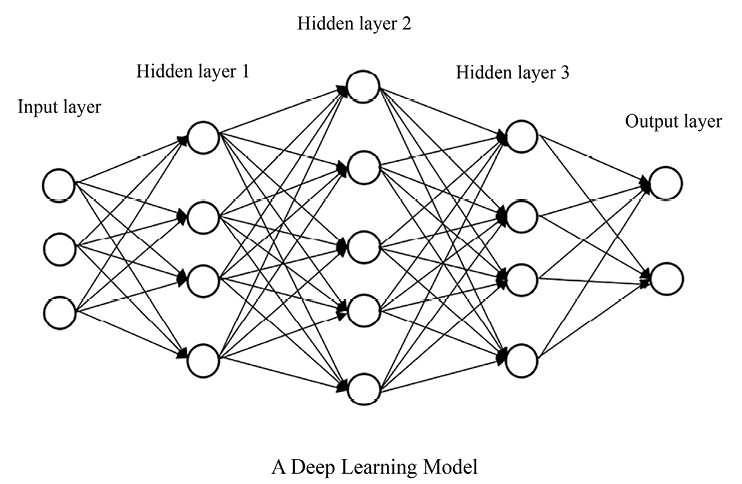
Figure 6.5: A deep neural network

In a stack of multiple hidden layers, the input of one hidden layer is the output of its previous layer, as you can see from Figure 6.5. Features (signals) are extracted from each hidden layer. Features from different layers represent patterns from different levels. Going beyond shallow neural networks (usually with only one hidden layer), a DL model (usually with two or more hidden layers) with the right network architectures and parameters can better learn complex non-linear relationships from data.

Let’s see some typical applications of DL so that you will be more motivated to get started with upcoming DL projects.

Computer vision is widely considered the area with massive breakthroughs in DL. You will learn more about this in Chapter 11, Categorizing Images of Clothing with Convolutional Neural Networks, and Chapter 14, Building an Image Search Engine Using CLIP: A Multimodal Approach. For now, here is a list of common applications in computer vision:

• Image recognition, such as face recognition and handwritten digit recognition. Handwritten digit recognition, along with the common evaluation dataset MNIST, has become a “Hello, World!” project in DL.
• Image-based search engines heavily utilize DL techniques in their image classification and image similarity encoding components.
• Machine vision, which is a critical part of autonomous vehicles, perceives camera views to make real-time decisions.
• Color restoration from black and white photos and art transfer that ingeniously blends two images of different styles. The artificial masterpieces in Google Arts & Culture (https://artsandculture.google.com/) are impressive.
• Realistic image generation based on textual descriptions. This has applications in creating visual storytelling content and assisting in content creation for marketing and advertising.

Natural Language Processing (NLP) is another field where you can see the dominant use of DL in its modern solutions. You will learn more about this in Chapter 12, Making Predictions with Sequences Using Recurrent Neural Networks, and Chapter 13, Advancing Language Understanding and Generation with the Transformer Models. But let’s quickly look at some examples now:

• Machine translation, where DL has dramatically improved accuracy and fluency, for example, the sentence-based Google Neural Machine Translation (GNMT) system.
• Text generation reproduces text by learning the intricate relationships between words in sentences and paragraphs with deep neural networks. You can become a virtual J. K. Rowling or Shakespeare if you train a model well on their works.
• Image captioning, also known as image-to-text, leverages deep neural networks to detect and recognize objects in images and “describe” those objects in a comprehensible sentence. It couples recent breakthroughs in computer vision and NLP. Examples can be found at https://cs.stanford.edu/people/karpathy/deepimagesent/generationdemo/ (developed by Andrej Karpathy from Stanford University).
• In other common NLP tasks such as sentiment analysis and information retrieval and extraction, DL models have achieved state-of-the-art performance.
• Artificial Intelligence-Generated Content (AIGC) is one of the recent breakthroughs. It uses DL technologies to create or assist in creating various types of content, such as articles, product descriptions, music, images, and videos.

Similar to shallow networks, we learn all the weights in a deep neural network using gradient descent with the goal of minimizing the MSE cost, J(W). And gradients, , are computed through backpropagation. The difference is that we backpropagate more than one hidden layer. In the next section, we will implement neural networks by starting with shallow networks and then moving on to deep ones.