Search icon CANCEL
Subscription
0
Cart icon
Your Cart (0 item)
Close icon
You have no products in your basket yet
Save more on your purchases! discount-offer-chevron-icon
Savings automatically calculated. No voucher code required.
Arrow left icon
Explore Products
Best Sellers
New Releases
Books
Videos
Audiobooks
Learning Hub
Free Learning
Arrow right icon
Arrow up icon
GO TO TOP
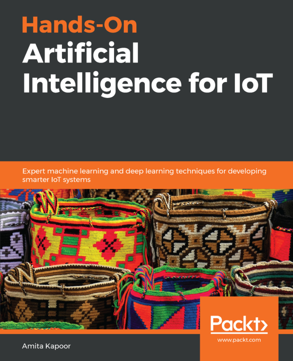
Hands-On Artificial Intelligence for IoT

You're reading from   Hands-On Artificial Intelligence for IoT Expert machine learning and deep learning techniques for developing smarter IoT systems

Arrow left icon
Product type Paperback
Published in Jan 2019
Publisher Packt
ISBN-13 9781788836067
Length 390 pages
Edition 2nd Edition
Languages
Arrow right icon
Author (1):
Arrow left icon
Dr. Amita Kapoor Dr. Amita Kapoor
Author Profile Icon Dr. Amita Kapoor
Dr. Amita Kapoor
Arrow right icon
View More author details
Toc

Table of Contents (14) Chapters Close

Preface 1. Principles and Foundations of IoT and AI FREE CHAPTER 2. Data Access and Distributed Processing for IoT 3. Machine Learning for IoT 4. Deep Learning for IoT 5. Genetic Algorithms for IoT 6. Reinforcement Learning for IoT 7. Generative Models for IoT 8. Distributed AI for IoT 9. Personal and Home IoT 10. AI for the Industrial IoT 11. AI for Smart Cities IoT 12. Combining It All Together 13. Other Books You May Enjoy

Tools used in this book

For the implementation of IoT-based services, we need to follow a bottom-up approach. For each IoT vertical, we need to find the analytics and the data and, finally, implement it in code.

Due to its availability in almost all AI and IoT platforms, Python will be used for coding in this book. Along with Python, some helping libraries such as NumPy, pandas, SciPy, Keras, and TensorFlow will be used to perform AI/ML analytics on the data. For visualization, we will be using Matplotlib and Seaborn.

TensorFlow

TensorFlow is an open source software library developed by the Google Brain team; it has functions and APIs for implementing deep neural networks. It works with Python, C++, Java, R, and Go. It can be used to work on multiple platforms, CPU, GPU, mobile, and even distributed. TensorFlow allows for model deployment and ease of use in production. The optimizer in TensorFlow makes the task of training deep neural networks easier by automatically calculating gradients and applying them to update weights and biases.

In TensorFlow, a program has two distinct components:

  • Computation graph is a network of nodes and edges. Here all of the data, variables, placeholders, and the computations to be performed are defined. TensorFlow supports three types of data objects: constants, variables, and placeholders.
  • Execution graph actually computes the network using a Session object. Actual calculations and transfer of information from one layer to another takes place in the Session object.

Let's see the code to perform matrix multiplication in TensorFlow. The whole code can be accessed from the GitHub repository (https://github.com/PacktPublishing/Hands-On-Artificial-Intelligence-for-IoT) filename, matrix_multiplication.ipynb:

import tensorflow as tf
import numpy as np

This part imports the TensorFlow module. Next, we define the computation graph. mat1 and mat2 are two matrices we need to multiply:

# A random matrix of size [3,5]
mat1 = np.random.rand(3,5)
# A random matrix of size [5,2]
mat2 = np.random.rand(5,2)

We declare two placeholders, A and B, so that we can pass their values at runtime. In the computation graph, we declare all of the data and computation objects:

# Declare placeholders for the two matrices 
A = tf.placeholder(tf.float32, None, name='A')
B = tf.placeholder(tf.float32, None, name='B')

This declares two placeholders with the names A and B; the arguments to the tf.placeholder method specify that the placeholders are of the float32 datatype. Since the shape specified is None, we can feed it a tensor of any shape and an optional name for the operation. Next, we define the operation to be performed using the matrix multiplication method, tf.matmul:

C = tf.matmul(A,B)

The execution graph is declared as a Session object, which is fed the two matrices, mat1 and mat2, for the placeholders, A and B, respectively:

with tf.Session() as sess:
result = sess.run(C, feed_dict={A: mat1, B:mat2})
print(result)

Keras

Keras is a high-level API that runs on top of TensorFlow. It allows for fast and easy prototyping. It supports both convolutional and recurrent neural networks, and even a combination of the two. It can run on both CPUs and GPUs. The following code performs matrix multiplication using Keras:

# Import the libraries
import keras.backend as K
import numpy as np

# Declare the data
A = np.random.rand(20,500)
B = np.random.rand(500,3000)

#Create Variable
x = K.variable(value=A)
y = K.variable(value=B)
z = K.dot(x,y)
print(K.eval(z))

Datasets

In the coming chapters, we'll be learning different DL models and ML methods. They all work on data; while a large number of datasets are available to demonstrate how these models work, in this book, we'll use datasets available freely through wireless sensors and other IoT devices. The following are some of the datasets used in this book and their sources.

The combined cycle power plant dataset

This dataset contains 9,568 data points collected from a combined cycle power plant (CCPP) in a course of six years (2006-2011). CCPP uses two turbines to generate power, the gas turbine and the steam turbine. There're three main components of the CCPP plant: gas turbine, heat recovery system, and steam turbine. The dataset, available at UCI ML (http://archive.ics.uci.edu/ml/datasets/combined+cycle+power+plant), was collected by Pinar Tufekci from Namik Kemal University and Heysem Kaya from Bogazici University. The data consists of four features determining the average ambient variables. The averages are taken from various sensors located around the plant that record ambient variables per second. The aim is to predict the net hourly electrical energy output. The data is available in both xls and ods formats.

The features in the dataset are as follows:

  • The Ambient Temperature (AT) is in the range 1.81°C and 37.11°C
  • The Ambient Pressure (AP) is in the range 992.89—1033.30 millibar
  • Relative Humidity (RH) is in the range 25.56% to 100.16%
  • Exhaust Vacuum (V) is in the range 25.36 to 81.56 cm Hg
  • Net hourly electrical energy output (PE) is in the range 420.26 to 495.76 MW
Further details about the data and the problem can be read from the following:
  • Pınar Tüfekci, Prediction of full load electrical power output of a baseload operated combined cycle power plant using machine learning methods, International Journal of Electrical Power & Energy Systems, Volume 60, September 2014, Pages 126-140, ISSN 0142-0615.
  • Heysem Kaya, Pınar Tüfekci, Sadık Fikret Gürgen: Local and GlobalLearning Methods for Predicting Power of a Combined Gas & Steam Turbine, Proceedings of the International Conference on Emerging Trends in Computer and Electronics Engineering ICETCEE 2012, pp. 13-18 (Mar. 2012, Dubai).

Wine quality dataset

Wineries around the world have to undergo wine certifications and quality assessments to safeguard human health. The wine certification is performed with the help of physicochemical analysis and sensory tests. With the advancement of technology, the physicochemical analysis can be performed routinely via in-vitro equipment.

We use this dataset for classification examples in this book. The dataset can be downloaded from the UCI-ML repository (https://archive.ics.uci.edu/ml/datasets/Wine+Quality). The wine quality dataset contains results of physicochemical tests on different samples of red and white wine. Each sample was further rated by an expert wine taster for quality on a scale of 0—10.

The dataset contains in total 4,898 instances; it has a total of 12 attributes. The 12 attributes are as follows:

  • Fixed acidity
  • Volatile acidity
  • Citric acid
  • Residual sugar
  • Chlorides
  • Free sulfur dioxide
  • Total sulfur dioxide
  • Density
  • pH
  • Sulfates
  • Alcohol
  • Quality

The dataset is available in the CSV format.

Details about the dataset can be read from this paper: Cortez, Paulo, et al. Modeling wine preferences by data mining from physicochemical properties. Decision Support Systems 47.4 (2009): 547-553 (https://repositorium.sdum.uminho.pt/bitstream/1822/10029/1/wine5.pdf).

Air quality data

Air pollution poses a major environmental risk to human health. It's found that there exists a correlation between improved air quality and amelioration of different health problems such as respiratory infections, cardiovascular diseases, and lung cancer. The extensive sensor networks throughout the world by Meteorological Organizations of the respective country provide us with real-time air quality data. This data can be accessed through the respective web APIs of these organizations.

In this book, we'll use the historical air quality data to train our network and predict the mortality rate. The historical data for England is available freely at Kaggle (https://www.kaggle.com/c/predict-impact-of-air-quality-on-death-rates), and the air quality data consists of daily means of ozone (O3), Nitrogen dioxide (NO2), particulate matter with a diameter less than or equal to 10 micrometers (PM10) and PM25 (2.5 micrometers or less), and temperature. The mortality rate (number of deaths per 100,000 people) for England region is obtained by the data provided by the UK Office for National Statistics.

You have been reading a chapter from
Hands-On Artificial Intelligence for IoT - Second Edition
Published in: Jan 2019
Publisher: Packt
ISBN-13: 9781788836067
Register for a free Packt account to unlock a world of extra content!
A free Packt account unlocks extra newsletters, articles, discounted offers, and much more. Start advancing your knowledge today.
Unlock this book and the full library FREE for 7 days
Get unlimited access to 7000+ expert-authored eBooks and videos courses covering every tech area you can think of
Renews at $19.99/month. Cancel anytime
Banner background image