Probabilistic forecasting with an LSTM

This recipe will walk you through building an LSTM neural network for probabilistic forecasting using PyTorch Lightning.

Getting ready

In this recipe, we’ll introduce probabilistic forecasting with LSTM networks. This approach combines the strengths of LSTM models in capturing long-term dependencies within sequential data with the nuanced perspective of probabilistic forecasting. This method goes beyond traditional point estimates by predicting a range of possible future outcomes, each accompanied by a probability. This means that we are incorporating uncertainty into forecasts.

This recipe uses the same dataset that we used in Chapter 4, in the Feedforward neural networks for multivariate time series forecasting recipe. We’ll also use the same data module we created in that recipe, which is called MultivariateSeriesDataModule.

Let’s explore how to use this data module to build an LSTM model for probabilistic forecasting.

How to do it…

In this subsection, we’ll define a probabilistic LSTM model that outputs the predictive mean and standard deviation for each forecasted point of the time series. This technique involves designing the LSTM model to predict parameters that define a probability distribution for future outcomes rather than outputting a single value. The model is usually configured to output parameters of a specific distribution, such as the mean and variance for a Gaussian distribution. These describe the expected value and the spread of future values, respectively:

1. Let’s start by defining a callback:

   class LossTrackingCallback(Callback):
       def __init__(self):
           self.train_losses = []
           self.val_losses = []
       def on_train_epoch_end(self, trainer, pl_module):
           if trainer.logged_metrics.get("train_loss_epoch"):
               self.train_losses.append(
                   trainer.logged_metrics["train_loss_epoch"].item())
       def on_validation_epoch_end(self, trainer, pl_module):
           if trainer.logged_metrics.get("val_loss_epoch"):
               self.val_losses.append(
                   trainer.logged_metrics["val_loss_epoch"].item())

   The LossTrackingCallback class is used to monitor the training and validation losses throughout the epochs. This is important for diagnosing the learning process of the model, identifying overfitting, and deciding when to stop training.

2. Then, we must build the LSTM model based on PyTorch Lightning’s LightningModule class:

   class ProbabilisticLSTM(LightningModule):
       def __init__(self, input_size,
                    hidden_size, seq_len,
                    num_layers=2):
           super().__init__()
           self.save_hyperparameters()
           self.lstm = nn.LSTM(input_size, hidden_size,
               num_layers, batch_first=True)
           self.fc_mu = nn.Linear(hidden_size, 1)
           self.fc_sigma = nn.Linear(hidden_size, 1)
           self.hidden_size = hidden_size
           self.softplus = nn.Softplus()
       def forward(self, x):
           lstm_out, _ = self.lstm(x)
           lstm_out = lstm_out[:, -1, :]
           mu = self.fc_mu(lstm_out)
           sigma = self.softplus(self.fc_sigma(lstm_out))
           return mu, sigma

   The ProbabilisticLSTM class defines the LSTM architecture for our probabilistic forecasts. The class includes layers to compute the predictive mean (fc_mu) and standard deviation (fc_sigma) of the forecast distribution. The standard deviation is passed through a Softplus() activation function to ensure it is always positive, reflecting the nature of standard deviation.

3. The following code implements the training and validation steps, along with the network configuration parameters:

       def training_step(self, batch, batch_idx):
           x, y = batch[0]["encoder_cont"], batch[1][0]
           mu, sigma = self.forward(x)
           dist = torch.distributions.Normal(mu, sigma)
           loss = -dist.log_prob(y).mean()
           self.log(
               "train_loss", loss, on_step=True,
               on_epoch=True, prog_bar=True, logger=True
           )
           return {"loss": loss, "log": {"train_loss": loss}}
       def validation_step(self, batch, batch_idx):
           x, y = batch[0]["encoder_cont"], batch[1][0]
           mu, sigma = self.forward(x)
           dist = torch.distributions.Normal(mu, sigma)
           loss = -dist.log_prob(y).mean()
           self.log(
               "val_loss", loss, on_step=True,
               on_epoch=True, prog_bar=True, logger=True
           )
           return {"val_loss": loss}
       def configure_optimizers(self):
           optimizer = optim.Adam(self.parameters(), lr=0.0001)
           scheduler = optim.lr_scheduler.ReduceLROnPlateau(
               optimizer, "min")
           return {
               "optimizer": optimizer,
               "lr_scheduler": scheduler,
               "monitor": "val_loss",
           }

4. After defining the model architecture, we initialize the data module and set up training callbacks. As we saw previously, the EarlyStopping callback is a valuable tool for preventing overfitting by halting the training process once the model ceases to improve on the validation set. The ModelCheckpoint callback ensures that we capture and save the best version of the model based on its validation performance. Together, these callbacks optimize the training process, aiding in developing a robust and well-tuned model:

   datamodule = ContinuousDataModule(data=mvtseries)
   datamodule.setup()
   model = ProbabilisticLSTM(
       input_size = input_size, hidden_size=hidden_size,
       seq_len=seq_len
   )
   early_stop_callback = EarlyStopping(monitor="val_loss", 
       patience=5)
   checkpoint_callback = ModelCheckpoint(
       dirpath="./model_checkpoint/", save_top_k=1, 
       monitor="val_loss"
   )
   loss_tracking_callback = LossTrackingCallback()
   trainer = Trainer(
       max_epochs=100,
       callbacks=[early_stop_callback, checkpoint_callback,
       loss_tracking_callback],
   )
   trainer.fit(model, datamodule)

   Using the Trainer class from PyTorch Lightning simplifies the training process, handling the complex training loops internally and allowing us to focus on defining the model and its behavior. It increases the code’s readability and maintainability, making experimenting with different model configurations easier.

5. After training, assessing the model’s performance and visualizing its probabilistic forecasts is very important. The graphical representation of the forecasted means, alongside their uncertainty intervals against the actual values, offers a clear depiction of the model’s predictive power and the inherent uncertainty in its predictions. We built a visualization framework to plot the forecasts. You can check the functions at the following link: https://github.com/PacktPublishing/Deep-Learning-for-Time-Series-Data-Cookbook.

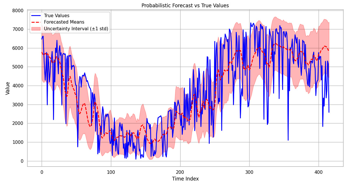
The following figure illustrates the true values of our time series in blue, with the forecasted means depicted by the dashed red line:

Figure 7.4: Probabilistic forecasts with uncertainty intervals and true values

The shaded area represents the uncertainty interval, calculated as a standard deviation from the forecasted mean. This probabilistic approach to forecasting provides a more comprehensive picture than point estimates as it accounts for the variability and uncertainty inherent in the time series data. The overlap between the uncertainty intervals and the actual values indicates areas where the model has higher confidence in its predictions. Conversely, wider intervals may suggest periods of more significant uncertainty, potentially due to inherent noise in the data or complex underlying dynamics that the model finds more challenging to capture.

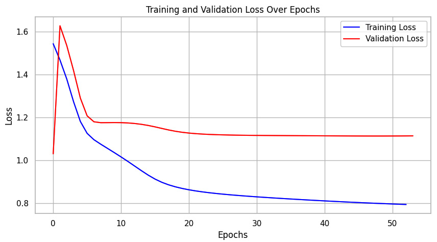
Moreover, the following figure provides insights into the training dynamics of our probabilistic LSTM model:

Figure 7.5: Training and validation loss over epochs, demonstrating the learning progress of the probabilistic LSTM model

The relatively stable and low validation loss suggests that our model generalizes well without overfitting the training data.

How it works…

The probabilistic LSTM model extends beyond traditional point prediction models. Unlike point forecasts, which output a single expected value, this model predicts a full distribution characterized by mean and standard deviation parameters.

This probabilistic approach provides a richer representation by capturing the uncertainty inherent in the data. The mean of the distribution gives the expected value of the forecast, while the standard deviation quantifies the confidence in the prediction, expressing the expected variability around the mean.

To train this model, we use a loss function that differs from those used in point prediction models. Instead of using MSE or MAE, which minimizes the difference between predicted and actual values, the probabilistic LSTM employs a negative log-likelihood loss function. This loss function, often called the probabilistic loss, maximizes the likelihood of the observed data under the predicted distribution.

This probabilistic loss function is particularly suited for uncertainty estimation as it directly penalizes the divergence between the predicted probability distribution and the observed values. When the predicted distribution assigns a high probability to the actual observed values, the negative log-likelihood is low, and thus the loss is low.