Setting up the plotting environment
Matplotlib is a Python package for data visualization. To get ourselves ready for Matplotlib plotting, we need to set up Python, install Matplotlib with its dependencies, as well as prepare a platform to execute and keep our running code. While Matplotlib provides a native GUI interface, we recommend using Jupyter Notebook. It allows us to run our code interactively while keeping the code, output figures, and any notes tidy. We will walk you through the setup procedure in this session.
Setting up Python
Matplotlib 2.0 supports both Python versions 2.7 and 3.4+. In this book, we will demonstrate using Python 3.4+. You can download Python from http://www.python.org/download/.
Windows
For Windows, Python is available as an installer or zipped source files. We recommend the executable installer because it offers a hassle-free installation. First, choose the right architecture. Then, simply follow the instructions. Usually, you will go with the default installation, which comes with the Python package manager pip and Tkinter standard GUI (Graphical User Interface) and adds Python to the PATH (important!). In just a few clicks, it's done!
Note
64-bit or 32-bit?
In most cases, you will go for the 64-bit (x86-64) version because it usually gives better performance. Most computers today are built with the 64-bit architecture, which allows more efficient use of system memory (RAM). Going on 64-bit means the processor reads data in larger chunks each time. It also allows more than 3 GB of data to be addressed. In scientific computing, we typically benefit from added RAM to achieve higher speed. Although using a 64-bit version doubles the memory footprint before exceeding the memory limit, it is often required for large data, such as in scientific computing. Of course, if you have a 32-bit computer, 32-bit is your only choice.
Using Python
- Press Win + R on the keyboard to call the
Rundialog. - Type
cmd.exein theRundialog to open Command Prompt:
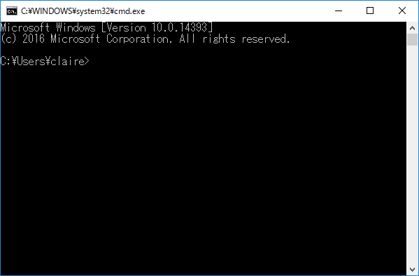
- In Command Prompt, type
python.
Note
For brevity, we will refer to both Windows Command Prompt and the Linux or Mac Terminal app as the "terminal" throughout this book.
Note
Some Python packages, such as Numpy and Scipy require Windows C++ compilers to work properly. We can obtain Microsoft Visual C++ compiler for free from the official site: http://landinghub.visualstudio.com/visual-cpp-build-tools As noted in the Python documentation page (https://wiki.python.org/moin/WindowsCompilers), a specific C++ compiler version is required for each Python version. Since most codes in this book were tested against Python 3.6, Microsoft Visual C++ 14.0 / Build Tools for Visual Studio 2017 is recommended. Readers can also check out Anaconda Python (https://www.continuum.io/downloads/), which ships with pre-built binaries for many Python packages. According to our experience, the Conda package manager resolves package dependencies in a much nicer way on Windows.
macOS
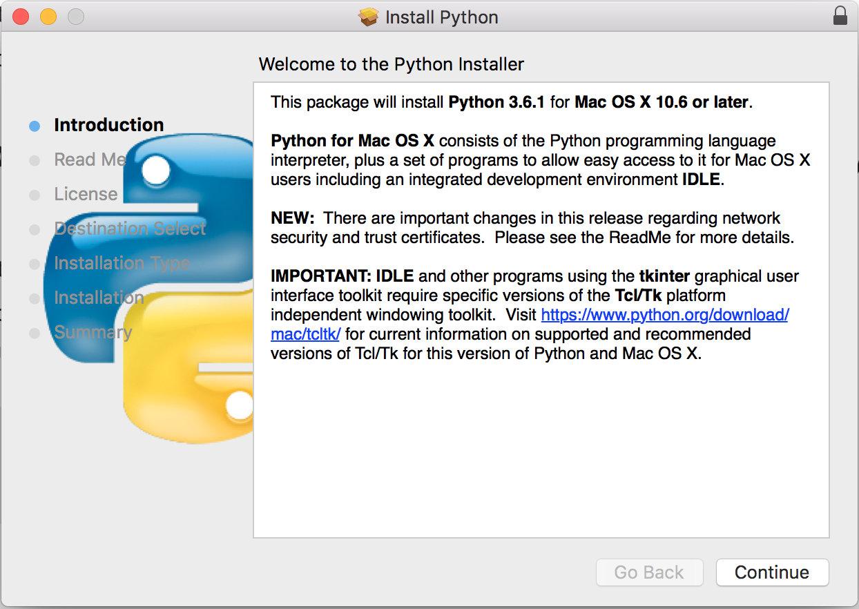
macOS comes with Python 2.7 installed. To ensure compatibility with the example code in this book, Python 3.4 or above is required, which is available for download from https://www.python.org/downloads/mac-osx/. You will be prompted by a graphical installation wizard when you run the downloaded installation package:
After completing the graphical installation steps, Python 3 can be accessed via these steps:
- Open the Finder app.
- Navigate to the
Applicationsfolder, and then go into theUtilitiesfolder. - Open the Terminal app.
- You will be prompted by the following message when you type
python3in the terminal:
Python 3.6.1 (v3.6.1:69c0db5, Mar 21 2017, 18:41:36 [GCC 4.2.1 (Apple Inc. build 5666) (dot 3)] on Darwin
Type "help", "copyright", "credits" or "license" for more information.
>>>
Note
Some Python packages require requires Xcode Command Line Tools to compile properly. Xcode can be obtained from Mac App Store. To install the command line tools, enter the following command in Terminal: xcode-select --install and follow the installation prompts.
Linux
Most recent Linux distributions come with Python 3.4+ preinstalled. You can check this out by typing python3 in the terminal. If Python 3 is installed, you should see the following message, which shows more information about the version:
Python 3.4.3 (default, Nov 17 2016, 01:08:31) [GCC 4.8.4] on Linux
Type "help", "copyright", "credits" or "license" for more information.
>>>
If Python 3 is not installed, you can install it on a Debian-based OS, such as Ubuntu, by running the following commands in the terminal:
sudo apt update
sudo apt install Python3 build-essential
The build-essential package contains compilers that are useful for building non-pure Python packages. You may need to substitute apt with apt-get if you have Ubuntu 14.04 or older.
Installing the Matplotlib dependencies
We recommend installing Matplotlib by a Python package manager, which will help you to automatically resolve and install dependencies upon each installation or upgrade of a package. We will demonstrate how to install Matplotlib with pip.
Installing the pip Python package manager
pip is installed with Python 2>=2.7.9 or Python 3>=3.4 binaries, but you will need to upgrade pip.
For the first time, you may do so by downloading get-pip.py from http://bootstrap.pypa.io/get-pip.py.
Then run this in the terminal:
python3 get-pip.pyYou can then type pip3 to run pip in the terminal.
After pip is installed, you may upgrade it by this command:
pip3 install –upgrade pipThe documentation of pip can be found at http://pip.pypa.io.
Installing Matplotlib with pip
To install Matplotlib with pip, simply type the following:
pip3 install matplotlibIt will automatically collect and install dependencies such as numpy.
Setting up Jupyter notebook
While Matplotlib offers a native plotting GUI, Jupyter notebook is a good option to execute and organize our code and output. We will soon introduce its advantages and usage.
Why Jupyter notebook?
Jupyter notebook (formerly known as IPython notebook) is an IPython-based interactive computational environment. Unlike the native Python console, code and imported data can easily be reused. There are also markdown functions that allow you to take notes like a real notebook. Code and other content can be separated into blocks (cells) for better organization. In particular, it offers a seamless integration with the matplotlib library for plot display.
Jupyter Notebook works as a server-client application and provides a neat web browser interface where you can edit and run your code. While you can run it locally even on a computer without internet access, notebooks on remote servers can be as easily accessed by SSH port forwarding. Multiple notebook instances, local or remote, can be run simultaneously on different network ports.
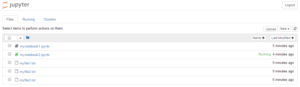
Here is a screenshot of a running Jupyter Notebook:
Jupyter notebook provides multiple saving options for easy sharing. There are also features such as auto-complete functions in the code editor that facilitate development.
In addition, Jupyter notebook offers different kernels to be installed for interactive computing with different programming languages. We will skip this for our purposes.
Installing Jupyter notebook
To install Jupyter notebook, simply type this in the terminal:
pip3 install jupyterUsing Jupyter notebook
Jupyter notebook is easy to use and can be accessed remotely as web pages on client browsers. Here is the basic usage of how to set up a new notebook session, run and save code, and jot down notes with the Markdown format.
Starting a Jupyter notebook session
- Type
jupyter notebookin the terminal or Command Prompt. - Open your favorite browser.
- Type in
localhost:8888as the URL.
To specify the port, such as when running multiple notebook instances on one or more machines, you can do so with the --port={port number} option.
For a notebook on remote servers, you can use SSH for port forwarding. Just specify the –L option with {port number}:localhost:{port number} during connection, as follows:
ssh –L 8888:localhost:8888 smith@remoteserverThe Jupyter Notebook home page will show up, listing files in your current directory. Notebook files are denoted by a book logo. Running notebooks are marked in green.
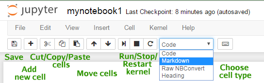
Editing and running code
A notebook contains boxes called cells. A new notebook begins with a gray box cell, which is a text area for code editing by default. To insert and edit code:
- Click inside the gray box.
- Type in your Python code.
- Click on the >| play button or press Shift + Enter to run the current cell and move the cursor to the next cell:
Cells can be run in different orders and rerun multiple times in a session. The output and any warnings or error messages are shown in the output area of each cell under each gray textbox. The number in square brackets on the left shows the order of the cell last run:
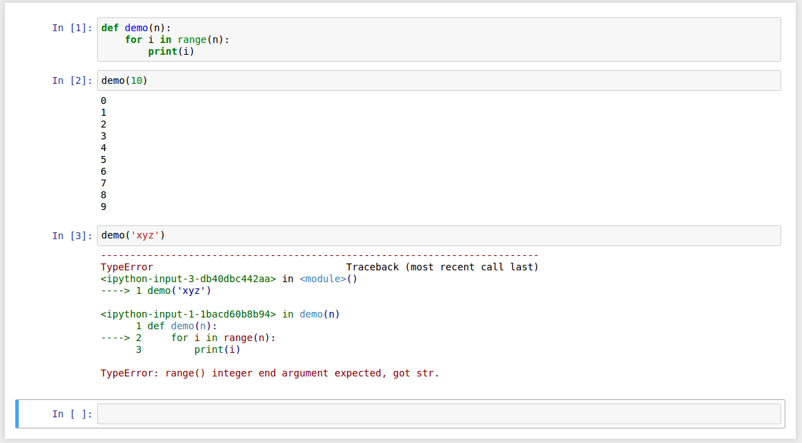
Once a cell is run, stored namespaces, including functions and variables, are shared throughout the notebook before the kernel restarts.
You can edit the code of any cells while some cells are running. If for any reason you want to interrupt the running kernel, such as to stop a loop that prints out too many messages, you can do so by clicking on the square interrupt button in the toolbar.
Note
Try not to print too much output when using Jupyter Notebook; it may crash your browser. However, long lists will be automatically abbreviated if you print them out.
Jotting down notes in Markdown mode
How do we insert words and style them to organize our notebook?
Here is the way:
- Select
Markdownfrom the drop-down list on the toolbar. - Type your notes in the gray box.
- Click on the >| play button or press Shift + Enter to display the markdown.
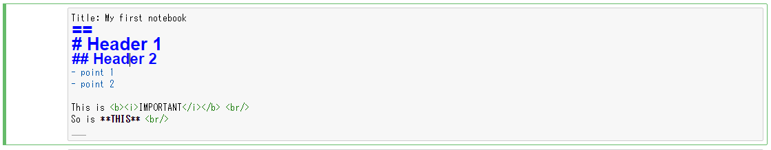
Markdown notation provides a handy way to style without much manual clicking or galore of tags:
Style | Method |
Headers: H1, H2, H3… | Start the line with a hash #, followed by a space, for example, # xxx, ## xxx, ### xxx. |
Title | Two or more equal signs on the next line, same effect as H1. |
Emphasis (italic) | *xxx* or _xxx_. |
Strong emphasis (bold) | **xxx** or __xxx__. |
Unordered list | Start each line with one of the markers: asterisk (*), minus (-), or plus (+). Then follow with a space, for example, * xxx. |
Ordered list | Start each line with ordered numbers from 1, followed by a period (.) and a space. |
Horizontal rule | Three underscores ___. |
A detailed cheatsheet is provided by Adam Pritchard at https://github.com/adam-p/markdown-here/wiki/Markdown-Cheatsheet.
Viewing Matplotlib plots
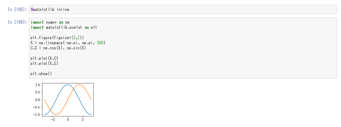
For static figures, type %matplotlib inline in a cell. The figure will be displayed in the output area:
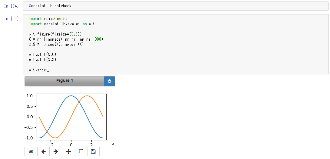
Running %matplotlib notebook will embed the Matplotlib interface in the output area.
Real-time interaction such as zooming and panning can be done under this mode. Clicking on the power sign button in the top-right corner will stop the interactive mode. The figure will become static, as in the case of %matplotlib inline:
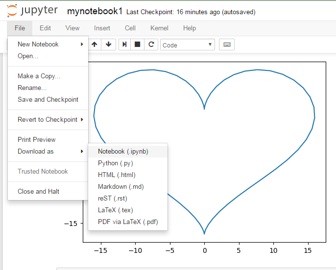
Saving the notebook project
Each notebook project can easily be saved and shared as the standard JSON-based .ipynb format (which can be run interactively by Jupyter on another machine), an ordinary .py Python script, or a static .html web page or .md format for viewing. To convert the notebook into Latex or .pdf via LaTeX files, Pandoc is required. More advanced users can check out the installation instructions of Pandoc on http://pandoc.org/installing.html:
All set to go!
We have now set up the necessary packages and learned the basic usage of our coding environment. Let’s start our journey!