Search icon CANCEL
Arrow left icon
Explore Products
Best Sellers
New Releases
Books
Videos
Audiobooks
Learning Hub
Conferences
Free Learning
Arrow right icon
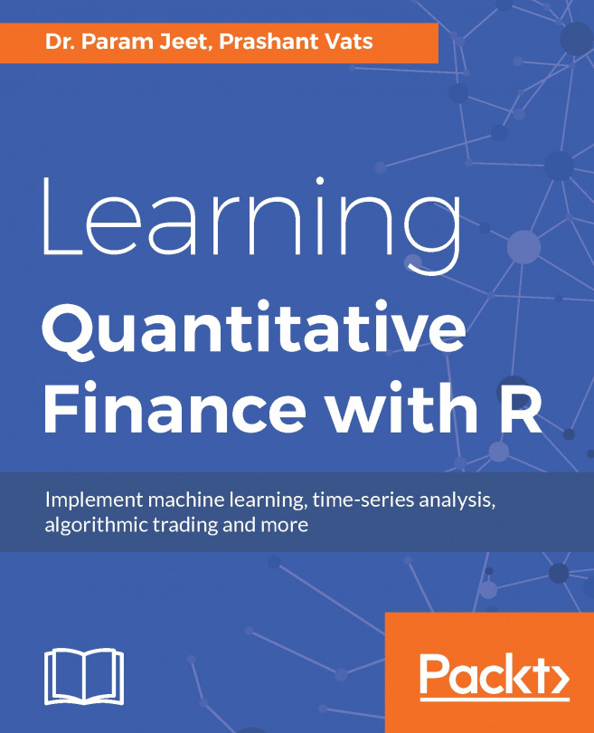
Learning Quantitative Finance with R

Learning Quantitative Finance with R: Implement machine learning, time-series analysis, algorithmic trading and more

eBook
$29.99 $43.99
Paperback
$54.99
Subscription
Free Trial
Renews at $19.99p/m

What do you get with eBook?

Product feature icon Instant access to your Digital eBook purchase
Product feature icon Download this book in EPUB and PDF formats
Product feature icon Access this title in our online reader with advanced features
Product feature icon DRM FREE - Read whenever, wherever and however you want
Table of content icon View table of contents Preview book icon Preview Book

Learning Quantitative Finance with R

Chapter 2. Statistical Modeling

In this chapter, we are going to discuss statistical modeling, which will be the first step in learning quantitative finance in R as the concepts of statistical modeling are the driving force for quantitative finance. Before starting this chapter, the assumption is that learners are familiar with basic programming in R and have a sound knowledge of statistical concepts. We will not be discussing statistical concepts in this chapter. We will be discussing how to do the statistical modeling in R.

This chapter covers the following topics:

  • Probability distributions
  • Sampling
  • Statistics
  • Correlation
  • Hypothesis testing
  • Parameter estimation
  • Outlier detection
  • Standardization
  • Normalization

Probability distributions

Probability distributions determine how the values of random variables are spread. For example, the set of all the possible outcomes of the tossing of a sequence of coins gives rise to binomial distribution. The means of large samples of the data population follow normal distribution, which is the most common and useful distribution.

The features of these distributions are very well known and can be used to extract inferences about the population. We are going to discuss in this chapter some of the most common probability distributions and how to compute them.

Normal distribution

Normal distribution is the most widely used probability distribution in the financial industry. It is a bell-shaped curve and mean, median mode is the same for normal distribution. It is denoted by Normal distribution where Normal distribution is the mean and Normal distribution  is the variance of the sample. If the mean is 0 and variance is 1 then the normal distribution is known as standard normal distribution N(1, 0).

Now let...

Sampling

When building any model in finance, we may have very large datasets on which model building will be very time-consuming. Once the model is built, if we need to tweak the model again, it is going to be a time-consuming process because of the volume of data. So it is better to get the random or proportionate sample of the population data on which model building will be easier and less time-consuming. So in this section, we are going to discuss how to select a random sample and a stratified sample from the data. This will play a critical role in building the model on sample data drawn from the population data.

Random sampling

Select the sample where all the observation in the population has an equal chance. It can be done in two ways, one without replacement and the other with replacement.

A random sample without replacement can be done by executing the following code:

> RandomSample <- Sampledata[sample(1:nrow(Sampledata), 10,  
>+ replace=FALSE),] 

This generates the following...

Statistics

In a given dataset, we try to summarize the data by the central position of the data, which is known as measure of central tendency or summary statistics. There are several ways to measure the central tendency, such as mean, median, and mode. Mean is the widely used measure of central tendency. Under different scenarios, we use different measures of central tendency. Now we are going to give an example of how to compute the different measures of central tendency in R.

Mean

mean is the equal weightage average of the sample. For example, we can compute the mean of Volume in the dataset Sampledata by executing the following code, which gives the arithmetic mean of the volume:

mean(Sampledata$Volume) 

Median

Median is the mid value of the matrix when it is arranged in a sorted way, which can be computed by executing the following code:

median(Sampledata$Volume) 

Mode

Mode is the value present in the attribute which has maximum frequency. For mode, there does not exist an inbuilt function...

Correlation

Correlation plays a very important role in quant finance. It not only determines the relation between the financial attributes but also plays a crucial role in predicting the future of financial instruments. Correlation is the measure of linear relationship between the two financial attributes. Now let us try to compute the different types of correlation in R using Sampledata, which is used in identifying the orders of components of predictive financial models.

Correlation can be computed by the following code. Let's first subset the data and then run the function for getting correlation:

x<-Sampledata[,2:5] 
rcorr(x, type="pearson") 

This generates the following correlation matrix, which shows the measure of linear relationship between the various daily level prices of a stock:

Open

High

Low

Close

Open

1

0.962062

0.934174

0.878553

High

0.962062

1

0.952676

0.945434

Low

0.934174

0.952676

1

0.960428

Close

0.878553

0.945434

...

Probability distributions


Probability distributions determine how the values of random variables are spread. For example, the set of all the possible outcomes of the tossing of a sequence of coins gives rise to binomial distribution. The means of large samples of the data population follow normal distribution, which is the most common and useful distribution.

The features of these distributions are very well known and can be used to extract inferences about the population. We are going to discuss in this chapter some of the most common probability distributions and how to compute them.

Normal distribution

Normal distribution is the most widely used probability distribution in the financial industry. It is a bell-shaped curve and mean, median mode is the same for normal distribution. It is denoted by  where  is the mean and  is the variance of the sample. If the mean is 0 and variance is 1 then the normal distribution is known as standard normal distribution N(1, 0).

Now let us discuss the main...

Sampling


When building any model in finance, we may have very large datasets on which model building will be very time-consuming. Once the model is built, if we need to tweak the model again, it is going to be a time-consuming process because of the volume of data. So it is better to get the random or proportionate sample of the population data on which model building will be easier and less time-consuming. So in this section, we are going to discuss how to select a random sample and a stratified sample from the data. This will play a critical role in building the model on sample data drawn from the population data.

Random sampling

Select the sample where all the observation in the population has an equal chance. It can be done in two ways, one without replacement and the other with replacement.

A random sample without replacement can be done by executing the following code:

> RandomSample <- Sampledata[sample(1:nrow(Sampledata), 10,  
>+ replace=FALSE),] 

This generates the...

Statistics


In a given dataset, we try to summarize the data by the central position of the data, which is known as measure of central tendency or summary statistics. There are several ways to measure the central tendency, such as mean, median, and mode. Mean is the widely used measure of central tendency. Under different scenarios, we use different measures of central tendency. Now we are going to give an example of how to compute the different measures of central tendency in R.

Mean

mean is the equal weightage average of the sample. For example, we can compute the mean of Volume in the dataset Sampledata by executing the following code, which gives the arithmetic mean of the volume:

mean(Sampledata$Volume) 

Median

Median is the mid value of the matrix when it is arranged in a sorted way, which can be computed by executing the following code:

median(Sampledata$Volume) 

Mode

Mode is the value present in the attribute which has maximum frequency. For mode, there does not exist an inbuilt...

Correlation


Correlation plays a very important role in quant finance. It not only determines the relation between the financial attributes but also plays a crucial role in predicting the future of financial instruments. Correlation is the measure of linear relationship between the two financial attributes. Now let us try to compute the different types of correlation in R using Sampledata, which is used in identifying the orders of components of predictive financial models.

Correlation can be computed by the following code. Let's first subset the data and then run the function for getting correlation:

x<-Sampledata[,2:5] 
rcorr(x, type="pearson") 

This generates the following correlation matrix, which shows the measure of linear relationship between the various daily level prices of a stock:

Open

High

Low

Close

Open

1

0.962062

0.934174

0.878553

High

0.962062

1

0.952676

0.945434

Low

0.934174

0.952676

1

0.960428

Close

0.878553

0.945434

0.960428...

Hypothesis testing


Hypothesis testing is used to reject or retain a hypothesis based upon the measurement of an observed sample. We will not be going into theoretical aspects but will be discussing how to implement the various scenarios of hypothesis testing in R.

Lower tail test of population mean with known variance

The null hypothesis is given by  where is the hypothesized lower bound of the population mean.

Let us assume a scenario where an investor assumes that the mean of daily returns of a stock since inception is greater than $10. The average of 30 days' daily return sample is $9.9. Assume the population standard deviation is 0.011. Can we reject the null hypothesis at .05 significance level?

Now let us calculate the test statistics z which can be computed by the following code in R:

> xbar= 9.9           
> mu0 = 10            
> sig = 1.1            
> n = 30                  
> z = (xbar-mu0)/(sig/sqrt(n))  
> z  

Here:

  • xbar: Sample...

Parameter estimates


In this section, we are going to discuss some of the algorithms used for parameter estimation.

Maximum likelihood estimation

Maximum likelihood estimation (MLE) is a method for estimating model parameters on a given dataset.

Now let us try to find the parameter estimates of a probability density function of normal distribution.

Let us first generate a series of random variables, which can be done by executing the following code:

> set.seed(100) 
> NO_values <- 100 
> Y <- rnorm(NO_values, mean = 5, sd = 1) 
> mean(Y) 

This gives 5.002913.

> sd(Y) 

This gives 1.02071.

Now let us make a function for log likelihood:

LogL <- function(mu, sigma) { 
+      A = dnorm(Y, mu, sigma) 
+      -sum(log(A)) 
+  } 

Now let us apply the function mle to estimate the parameters for estimating mean and standard deviation:

  > library(stats4) 
> mle(LogL, start = list(mu = 2, sigma=2)) 

mu and sigma have been...

Outlier detection


Outliers are very important to be taken into consideration for any analysis as they can make analysis biased. There are various ways to detect outliers in R and the most common one will be discussed in this section.

Boxplot

Let us construct a boxplot for the variable volume of the Sampledata, which can be done by executing the following code:

> boxplot(Sampledata$Volume, main="Volume", boxwex=0.1) 

The graph is as follows:

Figure 2.16: Boxplot for outlier detection

An outlier is an observation which is distant from the rest of the data. When reviewing the preceding boxplot, we can clearly see the outliers which are located outside the fences (whiskers) of the boxplot.

LOF algorithm

The local outlier factor (LOF) is used for identifying density-based local outliers. In LOF, the local density of a point is compared with that of its neighbors. If the point is in a sparser region than its neighbors then it is treated as an outlier. Let us consider some of the variables from...

Left arrow icon Right arrow icon
Download code icon Download Code

Key benefits

  • Understand the basics of R and how they can be applied in various Quantitative Finance scenarios
  • Learn various algorithmic trading techniques and ways to optimize them using the tools available in R.
  • Contain different methods to manage risk and explore trading using Machine Learning.

Description

The role of a quantitative analyst is very challenging, yet lucrative, so there is a lot of competition for the role in top-tier organizations and investment banks. This book is your go-to resource if you want to equip yourself with the skills required to tackle any real-world problem in quantitative finance using the popular R programming language. You'll start by getting an understanding of the basics of R and its relevance in the field of quantitative finance. Once you've built this foundation, we'll dive into the practicalities of building financial models in R. This will help you have a fair understanding of the topics as well as their implementation, as the authors have presented some use cases along with examples that are easy to understand and correlate. We'll also look at risk management and optimization techniques for algorithmic trading. Finally, the book will explain some advanced concepts, such as trading using machine learning, optimizations, exotic options, and hedging. By the end of this book, you will have a firm grasp of the techniques required to implement basic quantitative finance models in R.

Who is this book for?

If you want to learn how to use R to build quantitative finance models with ease, this book is for you. Analysts who want to learn R to solve their quantitative finance problems will also find this book useful. Some understanding of the basic financial concepts will be useful, though prior knowledge of R is not required.

What you will learn

  • Get to know the basics of R and how to use it in the field of Quantitative Finance
  • Understand data processing and model building using R
  • Explore different types of analytical techniques such as statistical analysis, time-series analysis, predictive modeling, and econometric analysis
  • Build and analyze quantitative finance models using real-world examples
  • How real-life examples should be used to develop strategies
  • Performance metrics to look into before deciding upon any model
  • Deep dive into the vast world of machine-learning based trading
  • Get to grips with algorithmic trading and different ways of optimizing it
  • Learn about controlling risk parameters of financial instruments

Product Details

Country selected
Publication date, Length, Edition, Language, ISBN-13
Publication date : Mar 23, 2017
Length: 284 pages
Edition : 1st
Language : English
ISBN-13 : 9781786465252
Category :
Languages :

What do you get with eBook?

Product feature icon Instant access to your Digital eBook purchase
Product feature icon Download this book in EPUB and PDF formats
Product feature icon Access this title in our online reader with advanced features
Product feature icon DRM FREE - Read whenever, wherever and however you want

Product Details

Publication date : Mar 23, 2017
Length: 284 pages
Edition : 1st
Language : English
ISBN-13 : 9781786465252
Category :
Languages :

Packt Subscriptions

See our plans and pricing
Modal Close icon
$19.99 billed monthly
Feature tick icon Unlimited access to Packt's library of 7,000+ practical books and videos
Feature tick icon Constantly refreshed with 50+ new titles a month
Feature tick icon Exclusive Early access to books as they're written
Feature tick icon Solve problems while you work with advanced search and reference features
Feature tick icon Offline reading on the mobile app
Feature tick icon Simple pricing, no contract
$199.99 billed annually
Feature tick icon Unlimited access to Packt's library of 7,000+ practical books and videos
Feature tick icon Constantly refreshed with 50+ new titles a month
Feature tick icon Exclusive Early access to books as they're written
Feature tick icon Solve problems while you work with advanced search and reference features
Feature tick icon Offline reading on the mobile app
Feature tick icon Choose a DRM-free eBook or Video every month to keep
Feature tick icon PLUS own as many other DRM-free eBooks or Videos as you like for just $5 each
Feature tick icon Exclusive print discounts
$279.99 billed in 18 months
Feature tick icon Unlimited access to Packt's library of 7,000+ practical books and videos
Feature tick icon Constantly refreshed with 50+ new titles a month
Feature tick icon Exclusive Early access to books as they're written
Feature tick icon Solve problems while you work with advanced search and reference features
Feature tick icon Offline reading on the mobile app
Feature tick icon Choose a DRM-free eBook or Video every month to keep
Feature tick icon PLUS own as many other DRM-free eBooks or Videos as you like for just $5 each
Feature tick icon Exclusive print discounts

Frequently bought together


Stars icon
Total $ 164.97
Python for Finance
$54.99
Mastering R for Quantitative Finance
$54.99
Learning Quantitative Finance with R
$54.99
Total $ 164.97 Stars icon

Table of Contents

9 Chapters
1. Introduction to R Chevron down icon Chevron up icon
2. Statistical Modeling Chevron down icon Chevron up icon
3. Econometric and Wavelet Analysis Chevron down icon Chevron up icon
4. Time Series Modeling Chevron down icon Chevron up icon
5. Algorithmic Trading Chevron down icon Chevron up icon
6. Trading Using Machine Learning Chevron down icon Chevron up icon
7. Risk Management Chevron down icon Chevron up icon
8. Optimization Chevron down icon Chevron up icon
9. Derivative Pricing Chevron down icon Chevron up icon

Customer reviews

Rating distribution
Full star icon Full star icon Full star icon Half star icon Empty star icon 3.7
(3 Ratings)
5 star 66.7%
4 star 0%
3 star 0%
2 star 0%
1 star 33.3%
Manuel Amunategui Mar 31, 2017
Full star icon Full star icon Full star icon Full star icon Full star icon 5
I’d like to recommend this book to those looking for wide coverage on quantitative finance using the R language (but I am biased as I was the technical reviewer for the book :-) For those who know me and my blog (amunategui.github.io), know that I always appreciate easy to understand language and lots of hands-on examples, and this book is built on such foundation.This book offers a great overview of many R libraries covering topics from financial probability and modeling all the way to trading, derivatives, and risk management - and my personal favorites - algorithmic trading and derivative pricing.
Amazon Verified review Amazon
Amazon Customer Aug 21, 2018
Full star icon Full star icon Full star icon Full star icon Full star icon 5
Very nicely written book and easy to understand. I received the book today and gone through the first chapter it is really easy to understand as an amateur in the field of R. Thanks to the authors who wrote the book from the beginner's perspective. One thing that must be added with the book is the CD for the exercises.
Amazon Verified review Amazon
Lindarden07 Sep 23, 2017
Full star icon Empty star icon Empty star icon Empty star icon Empty star icon 1
This book gives a list of functions for each topic. No detailed explanation is given. It serves as a reference to see which package and function you need to use to address some problems you are facing. But for detailed content, look for somewhere else.
Amazon Verified review Amazon
Get free access to Packt library with over 7500+ books and video courses for 7 days!
Start Free Trial

FAQs

How do I buy and download an eBook? Chevron down icon Chevron up icon

Where there is an eBook version of a title available, you can buy it from the book details for that title. Add either the standalone eBook or the eBook and print book bundle to your shopping cart. Your eBook will show in your cart as a product on its own. After completing checkout and payment in the normal way, you will receive your receipt on the screen containing a link to a personalised PDF download file. This link will remain active for 30 days. You can download backup copies of the file by logging in to your account at any time.

If you already have Adobe reader installed, then clicking on the link will download and open the PDF file directly. If you don't, then save the PDF file on your machine and download the Reader to view it.

Please Note: Packt eBooks are non-returnable and non-refundable.

Packt eBook and Licensing When you buy an eBook from Packt Publishing, completing your purchase means you accept the terms of our licence agreement. Please read the full text of the agreement. In it we have tried to balance the need for the ebook to be usable for you the reader with our needs to protect the rights of us as Publishers and of our authors. In summary, the agreement says:

  • You may make copies of your eBook for your own use onto any machine
  • You may not pass copies of the eBook on to anyone else
How can I make a purchase on your website? Chevron down icon Chevron up icon

If you want to purchase a video course, eBook or Bundle (Print+eBook) please follow below steps:

  1. Register on our website using your email address and the password.
  2. Search for the title by name or ISBN using the search option.
  3. Select the title you want to purchase.
  4. Choose the format you wish to purchase the title in; if you order the Print Book, you get a free eBook copy of the same title. 
  5. Proceed with the checkout process (payment to be made using Credit Card, Debit Cart, or PayPal)
Where can I access support around an eBook? Chevron down icon Chevron up icon
  • If you experience a problem with using or installing Adobe Reader, the contact Adobe directly.
  • To view the errata for the book, see www.packtpub.com/support and view the pages for the title you have.
  • To view your account details or to download a new copy of the book go to www.packtpub.com/account
  • To contact us directly if a problem is not resolved, use www.packtpub.com/contact-us
What eBook formats do Packt support? Chevron down icon Chevron up icon

Our eBooks are currently available in a variety of formats such as PDF and ePubs. In the future, this may well change with trends and development in technology, but please note that our PDFs are not Adobe eBook Reader format, which has greater restrictions on security.

You will need to use Adobe Reader v9 or later in order to read Packt's PDF eBooks.

What are the benefits of eBooks? Chevron down icon Chevron up icon
  • You can get the information you need immediately
  • You can easily take them with you on a laptop
  • You can download them an unlimited number of times
  • You can print them out
  • They are copy-paste enabled
  • They are searchable
  • There is no password protection
  • They are lower price than print
  • They save resources and space
What is an eBook? Chevron down icon Chevron up icon

Packt eBooks are a complete electronic version of the print edition, available in PDF and ePub formats. Every piece of content down to the page numbering is the same. Because we save the costs of printing and shipping the book to you, we are able to offer eBooks at a lower cost than print editions.

When you have purchased an eBook, simply login to your account and click on the link in Your Download Area. We recommend you saving the file to your hard drive before opening it.

For optimal viewing of our eBooks, we recommend you download and install the free Adobe Reader version 9.