Cross-Validation: Choosing the Regularization Parameter
By now, you may suspect that we could use regularization in order to decrease the overfitting we observed when we tried to model the synthetic data in Exercise 4.02, Generating and Modeling Synthetic Classification Data. The question is, how do we choose the regularization parameter, C? C is an example of a model hyperparameter. Hyperparameters are different from the parameters that are estimated when a model is trained, such as the coefficients and the intercept of a logistic regression. Rather than being estimated by an automated procedure like the parameters are, hyperparameters are input directly by the user as keyword arguments, typically when instantiating the model class. So, how do we know what values to choose?
Hyperparameters are more difficult to estimate than parameters. This is because it is up to the data scientist to determine what the best value is, as opposed to letting an optimization algorithm find it. However, it is possible to programmatically choose hyperparameter values, which could be viewed as an optimization procedure in its own right. Practically speaking, in the case of the regularization parameter C, this is most commonly done by fitting the model on one set of data with a particular value of C, determining model training performance, and then assessing the out-of-sample performance on another set of data.
We are already familiar with the concept of using model training and test sets. However, there is a key difference here; for instance, what would happen if we were to use the test set multiple times in order to see the effect of different values of C?
It may occur to you that after the first time you use the unseen test set to assess the out-of-sample performance for a particular value of C, it is no longer an "unseen" test set. While only the training data was used for estimating the model parameters (that is, the coefficients and the intercept), now the test data is being used to estimate the hyperparameter C. Effectively, the test data has now become additional training data in the sense that it is being used to find a good value for the hyperparameter.
For this reason, it is common to divide the data into three parts: a training set, a test set, and a validation set. The validation set serves multiple purposes:
Estimating Hyperparameters
The validation set can be repeatedly used to assess the out-of-sample performance with different hyperparameter values to select hyperparameters.
A Comparison of Different Models
In addition to finding hyperparameter values for a model, the validation set can be used to estimate the out-of-sample performance of different models; for example, if we wanted to compare logistic regression to random forest.
Note
Data Management Best Practices
As a data scientist, it's up to you to figure out how to divide up your data for different predictive modeling tasks. In the ideal case, you should reserve a portion of your data for the very end of the process, after you've already selected model hyperparameters and also selected the best model. This unseen test set is reserved for the last step, when it can be used to assess the endpoint of your model-building efforts, to see how the final model generalizes to new unseen data. When reserving the test set, it is good practice to make sure that the features and responses have similar characteristics to the rest of the data. In other words, the class fraction should be the same, and the distribution of features should be similar. This way, the test data should be representative of the data you built the model with.
While model validation is a good practice, it raises the question of whether the particular split we choose for the training, validation, and test data has any effect on the outcomes that we are tracking. For example, perhaps the relationship between the features and the response variable is slightly different in the unseen test set that we have reserved, or in the validation set, versus the training set. It is likely impossible to eliminate all such variability, but we can use the method of cross-validation to avoid placing too much faith in one particular split of the data.
Scikit-learn provides convenient functions to facilitate cross-validation analyses. These functions play a similar role to train_test_split, which we have already been using, although the default behavior is somewhat different. Let's get familiar with them now. First, import these two classes:
from sklearn.model_selection import StratifiedKFold
from sklearn.model_selection import KFold
Similar to train_test_split, we need to specify what proportion of the dataset we would like to use for training versus testing. However, with cross-validation (specifically the k-fold cross-validation that was implemented in the classes we just imported), rather than specifying a proportion directly, we simply indicate how many folds we would like – that is, the "k folds." The idea here is that the data will be divided into k equal proportions. For example, if we specify 4 folds, then each fold will have 25% of the data. These folds will be the test data in four separate instances of model training, while the remaining 75% from each fold will be used to train the model. In this procedure, each data point gets used as training data a total of k - 1 times, and as test data only once.
When instantiating the class, we indicate the number of folds, whether or not to shuffle the data before splitting, and a random seed if we want repeatable results across different runs:
n_folds = 4
k_folds = KFold(n_splits=n_folds, shuffle=False)
Here, we've instantiated an object with four folds and no shuffling. The way in which we use the object that is returned, which we've called k_folds, is by passing the features and response data that we wish to use for cross-validation, to the .split method of this object. This outputs an iterator, which means that we can loop through the output to get the different splits of training and test data. If we took the training data from our synthetic classification problem, X_syn_train and y_syn_train, we could loop through the splits like this:
for train_index, test_index in k_folds_iterator.split(X_syn_train,
                                                      y_syn_train):
The iterator will return the row indices of X_syn_train and y_syn_train, which we can use to index the data. Inside this for loop, we can write code to use these indices to select data for repeatedly training and testing a model object with different subsets of the data. In this way, we can get a robust indication of the out-of-sample performance when using one particular hyperparameter value, and then repeat the whole process using another hyperparameter value. Consequently, the cross-validation loop may sit nested inside an outer loop over different hyperparameter values. We'll illustrate this in the following exercise.
First though, what do these splits look like? If we were to simply plot the indices from train_index and test_index as different colors, we would get something that looks like this:
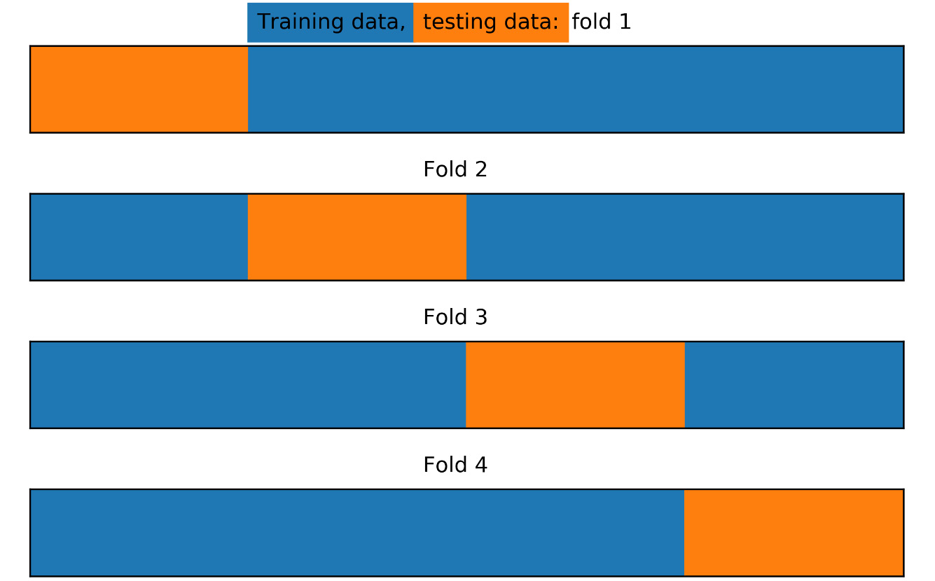
Figure 4.17: Training/test splits for k-folds with four folds and no shuffling
Here, we see that with the options we've indicated for the KFold class, the procedure has simply taken the first 25% of the data, according to the order of rows, as the first test fold, then the next 25% of data for the second fold, and so on. But what if we wanted stratified folds? In other words, what if we wanted to ensure that the class fractions of the response variable were equal in every fold? While train_test_split allows this option as a keyword argument, there is a separate StratifiedKFold class that implements this for cross-validation. We can illustrate how the stratified splits will appear as follows:
k_folds = StratifiedKFold(n_splits=n_folds, shuffle=False)
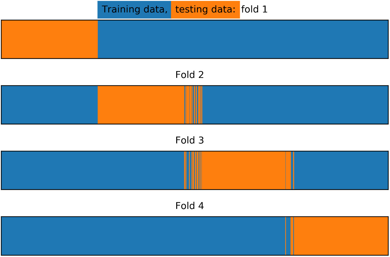
Figure 4.18: Training/test splits for stratified k-folds
In Figure 4.18, we can see that there has been some amount of "shuffling" between the different folds. The procedure has moved samples between folds as necessary to ensure that the class fractions in each fold are equal.
Now, what if we want to shuffle the data to choose samples from throughout the range of indices for each test fold? First, why might we want to do this? Well, with the synthetic data that we've created for our problem, we can be certain that the data is in no particular order. However, in many real-world situations, the data we receive may be sorted in some way.
For instance, perhaps the rows of the data have been ordered by the date an account was created, or by some other logic. Therefore, it can be a good idea to shuffle the data before splitting. This way, any traits that might have been used for sorting can be expected to be consistent throughout the folds. Otherwise, the data in different folds may have different characteristics, possibly leading to different relationships between features and response.
This can lead to a situation where model performance is uneven between the folds. In order to "mix up" the folds throughout all the row indices of a dataset, all we need to do is set the shuffle parameter to True:
k_folds = StratifiedKFold(n_splits=n_folds, shuffle=True,
                          random_state=1)
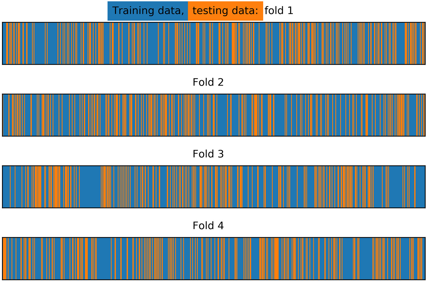
Figure 4.19: Training/test splits for stratified k-folds with shuffling
With shuffling, the test folds are spread out randomly, and fairly evenly, across the indices of the input data.
K-fold cross-validation is a widely used method in data science. However, the choice of how many folds to use depends on the particular dataset at hand. Using a smaller number of folds means that the amount of training data in each fold will be relatively small. Therefore, this increases the chances that the model will underfit, as models generally work better when trained on more data. It's a good idea to try a few different numbers of folds and see how the mean and the variability of the k-fold test score changes. Common numbers of folds can range anywhere from 4 or 5 to 10.
In the event of a very small dataset, it may be necessary to use as much data as possible for training in the cross-validation folds. In this scenario, you can use a method called leave-one-out cross-validation (LOOCV). In LOOCV, the test set for each fold consists of a single sample. In other words, there will be as many folds as there are samples in the training data. For each iteration, the model is trained on all but one sample, and a prediction is made for that sample. The accuracy, or other performance metric, can then be constructed using these predictions.
Other concerns that relate to the creation of a test set, such as choosing an out-of-time test set for problems where observations from the past must be used to predict future events, also apply to cross-validation.
In Exercise 4.02, Generating and Modeling Synthetic Classification Data, we saw that fitting a logistic regression on our training data led to overfitting. Indeed, the test score (ROC AUC = 0.81) was substantially lower than the training score (ROC AUC = 0.94). We had essentially used very little or no regularization by setting the regularization parameter C to a relatively large value (1,000). Now we will see what happens when we vary C through a wide range of values.
Note
The code for generating the plots presented in this section can be found here: https://packt.link/37Zks.
Exercise 4.03: Reducing Overfitting on the Synthetic Data Classification Problem
This exercise is a continuation of Exercise 4.02, Generating and Modeling Synthetic Classification Data. Here, we will use a cross-validation procedure in order to find a good value for the hyperparameter C. We will do this by using only the training data, reserving the test data for after model building is complete. Be prepared – this is a long exercise – but it will illustrate a general procedure that you will be able to use with many different kinds of machine learning models, so it is worth the time spent here. Perform the following steps to complete the exercise:
Note
Before you begin this exercise, you need to execute some prerequisite steps that can be found in the following notebook along with the code for this exercise: https://packt.link/JqbsW.
- Vary the value of the regularization parameter, C, to range from C = 1000 to C = 0.001. You can use the following snippets to do this.
First, define exponents, which will be powers of 10, as follows:
C_val_exponents = np.linspace(3,-3,13)
C_val_exponents
Here is the output of the preceding code:
array([ 3. , 2.5, 2. , 1.5, 1. , 0.5, 0. , -0.5, -1. , -1.5, -2. , -2.5, -3. ])
Now, vary C by the powers of 10, as follows:
C_vals = np.float(10)**C_val_exponents
C_vals
Here is the output of the preceding code:
array([1.00000000e+03, 3.16227766e+02, 1.00000000e+02, 3.16227766e+01,
       1.00000000e+01, 3.16227766e+00, 1.00000000e+00, 3.16227766e-01,
       1.00000000e-01, 3.16227766e-02, 1.00000000e-02, 3.16227766e-03,
       1.00000000e-03])
It's generally a good idea to vary the regularization parameter by powers of 10, or by using a similar strategy, as training models can take a substantial amount of time, especially when using k-fold cross-validation. This gives you a good idea of how a wide range of C values impacts the bias-variance trade-off, without needing to train a very large number of models. In addition to the integer powers of 10, we also include points on the log10 scale that are about halfway between. If it seems like there is some interesting behavior in between these relatively widely spaced values, you can add more granular values for C in a smaller part of the range of possible values.
- Import the
roc_curveclass:from sklearn.metrics import roc_curve
We'll continue to use the ROC AUC score for assessing, training, and testing performance. Now that we have several values of C to try and several folds (in this case four) for the cross-validation, we will want to store the training and test scores for each fold and for each value of C.
- Define a function that takes the
k_foldscross-validation splitter, the array of C values (C_vals), the model object (model), and the features and response variable (XandY, respectively) as inputs, to explore different amounts of regularization with k-fold cross-validation. Use the following code:def cross_val_C_search(k_folds, C_vals, model, X, Y):
Note
The function we started in this step will return the ROC AUCs and ROC curve data. The return block will be written during a later step in the exercise. For now, you can simply write the preceding code as is, because we will be defining
k_folds,C_vals,model,X, andYas we progress in the exercise. - Within this function block, create a NumPy array to hold model performance data, with dimensions
n_foldsbylen(C_vals):n_folds = k_folds.n_splits cv_train_roc_auc = np.empty((n_folds, len(C_vals))) cv_test_roc_auc = np.empty((n_folds, len(C_vals)))
Next, we'll store the arrays of true and false positive rates and thresholds that go along with each of the test ROC AUC scores in a list of lists.
Note
This is a convenient way to store all this model performance information, as a list in Python can contain any kind of data, including another list. Here, each item of the inner lists in the list of lists will be a tuple holding the arrays of TPR, FPR, and the thresholds for each of the folds, for each of the C values. Tuples are an ordered collection data type in Python, similar to lists, but unlike lists they are immutable: the items in a tuple can't be changed after the tuple is created. When a function returns multiple values, like the roc_curve function of scikit-learn, these values can be output to a single variable, which will be a tuple of those values. This way of storing results should be more obvious when we access these arrays later in order to examine them.
- Create a list of empty lists using
[[]]and*len(C_vals)as follows:cv_test_roc = [[]]*len(C_vals)
Using
*len(C_vals)indicates that there should be a list of tuples of metrics (TPR, FPR, thresholds) for each value of C.We have learned how to loop through the different folds for cross-validation in the preceding section. What we need to do now is write an outer loop in which we will nest the cross-validation loop.
- Create an outer loop for training and testing each of the k-folds for each value of C:
for c_val_counter in range(len(C_vals)):
    #Set the C value for the model object
    model.C = C_vals[c_val_counter]
    #Count folds for each value of C
    fold_counter = 0
We can reuse the same model object that we have already, and simply set a new value of C within each run of the loop. Inside the loop of C values, we run the cross-validation loop. We begin by yielding the training and test data row indices for each split.
- Obtain the training and test indices for each fold:
for train_index, test_index in k_folds.split(X, Y):
- Index the features and response variable to obtain the training and test data for this fold using the following code:
X_cv_train, X_cv_test = X[train_index], X[test_index]
y_cv_train, y_cv_test = Y[train_index], Y[test_index]
The training data for the current fold is then used to train the model.
- Fit the model on the training data, as follows:
model.fit(X_cv_train, y_cv_train)
This will effectively "reset" the model from whatever the previous coefficients and intercept were to reflect the training on this new data.
The training and test ROC AUC scores are then obtained, as well as the arrays of TPRs, FPRs, and thresholds that go along with the test data.
- Obtain the training ROC AUC score:
y_cv_train_predict_proba = model.predict_proba(X_cv_train)
cv_train_roc_auc[fold_counter, c_val_counter] = \
roc_auc_score(y_cv_train, y_cv_train_predict_proba[:,1])
- Obtain the test ROC AUC score:
y_cv_test_predict_proba = model.predict_proba(X_cv_test)
cv_test_roc_auc[fold_counter, c_val_counter] = \
roc_auc_score(y_cv_test, y_cv_test_predict_proba[:,1])
- Obtain the test ROC curves for each fold using the following code:
this_fold_roc = roc_curve(y_cv_test, y_cv_test_predict_proba[:,1])
cv_test_roc[c_val_counter].append(this_fold_roc)
We will use a fold counter to keep track of the folds that are incremented, and once outside the cross-validation loop, we print a status update to standard output. Whenever performing long computational procedures, it's a good idea to periodically print the status of the job so that you can monitor its progress and confirm that things are still working correctly. This cross-validation procedure will likely take only a few seconds on your laptop, but for longer jobs this can be especially reassuring.
- Increment the fold counter using the following code:
fold_counter += 1
- Write the following code to indicate the progress of execution for each value of C:
print('Done with C = {}'.format(lr_syn.C)) - Write the code to return the ROC AUCs and ROC curve data and finish the function:
return cv_train_roc_auc, cv_test_roc_auc, cv_test_roc
Note that we will continue to use the split into four folds that we illustrated previously, but you are encouraged to try this procedure with different numbers of folds to compare the effect.
We have covered a lot of material in the preceding steps. You may want to take a few moments to review this with your classmates in order to make sure that you understand each part. Running the function is comparatively simple. That is the beauty of a well-designed function – all the complicated parts get abstracted away, allowing you to concentrate on usage.
- Run the function we've designed to examine cross-validation performance, with the C values that we previously defined, and by using the model and data we were working with in the previous exercise. Use the following code:
cv_train_roc_auc, cv_test_roc_auc, cv_test_roc = \
cross_val_C_search(k_folds, C_vals, lr_syn, X_syn_train, y_syn_train)
When you run this code, you should see the following output populate below the code cell as the cross-validation is completed for each value of C:
Done with C = 1000.0
Done with C = 316.22776601683796
Done with C = 100.0
Done with C = 31.622776601683793
Done with C = 10.0
Done with C = 3.1622776601683795
Done with C = 1.0
Done with C = 0.31622776601683794
Done with C = 0.1
Done with C = 0.03162277660168379
Done with C = 0.01
Done with C = 0.0031622776601683794
Done with C = 0.001
So, what do the results of the cross-validation look like? There are a few ways to examine this. It is useful to look at the performance of each fold individually, so that you can see how variable the results are.
This tells you how different subsets of your data perform as test sets, leading to a general idea of the range of performance you can expect from the unseen test set. What we're interested in here is whether or not we are able to use regularization to alleviate the overfitting that we saw. We know that using C = 1,000 led to overfitting – we know this from comparing the training and test scores. But what about the other C values that we've tried? A good way to visualize this will be to plot the training and test scores on the y-axis and the values of C on the x-axis.
- Loop over each of the folds to view their results individually by using the following code:
for this_fold in range(k_folds.n_splits):
    plt.plot(C_val_exponents, cv_train_roc_auc[this_fold], '-o',\
             color=cmap(this_fold),\
             label='Training fold {}'.format(this_fold+1))
    plt.plot(C_val_exponents, cv_test_roc_auc[this_fold], '-x',\
             color=cmap(this_fold),\
             label='Testing fold {}'.format(this_fold+1))
plt.ylabel('ROC AUC')
plt.xlabel('log$_{10}$(C)')
plt.legend(loc = [1.1, 0.2])
plt.title('Cross validation scores for each fold')
You will obtain the following output:

Figure 4.20: The training and test scores for each fold and C-value
We can see that for each fold of the cross-validation, as C decreases, the training performance also decreases. However, at the same time, the test performance increases. For some folds and values of C, the test ROC AUC score actually exceeds that of the training data, while for others, these two metrics simply come closer together. In all cases, we can say that the C values of 10-1.5 and 10-2 appear to have a similar test performance, which is substantially higher than the test performance of C = 103. So, it appears that regularization has successfully addressed our overfitting problem.
But what about the lower values of C? For values that are lower than 10-2, the ROC AUC metric suddenly drops to 0.5. As you know, this value means that the classification model is essentially useless, performing no better than a coin flip. You are encouraged to check on this later when exploring how regularization affects the coefficient values; however, this is what happens when so much L1 regularization is applied that all model coefficients shrink to 0. Obviously, such models are not useful to us, as they encode no information about the relationship between the features and response variable.
Looking at the training and test performance of each k-fold split is helpful for gaining insights into the variability of model performance that may be expected when the model is scored on new, unseen data. But in order to summarize the results of the k-folds procedure, a common approach is to average the performance metric over the folds, for each value of the hyperparameter being considered. We'll perform this in the next step.
- Plot the mean of training and test ROC AUC scores for each C value using the following code:
plt.plot(C_val_exponents, np.mean(cv_train_roc_auc, axis=0), \
         '-o', label='Average training score')
plt.plot(C_val_exponents, np.mean(cv_test_roc_auc, axis=0), \
         '-x', label='Average testing score')
plt.ylabel('ROC AUC')
plt.xlabel('log$_{10}$(C)')
plt.legend()
plt.title('Cross validation scores averaged over all folds')
Figure 4.21: The average training and test scores across cross-validation folds
From this plot, it's clear that C = 10-1.5 and 10-2 are the best values of C. There is little or no overfitting here, as the average training and test scores are nearly the same. You could search a finer grid of C values (that is C = 10-1.1, 10-1.2, and so on) in order to more precisely locate a C value. However, from our graph, we can see that either C = 10-1.5 or C = 10-2 will likely be good solutions. We will move forward with C = 10-1.5.
Examining the summary metric of ROC AUC is a good way to get a quick idea of how models will perform. However, for any real-world business application, you will often need to choose a specific threshold, which goes along with specific true and false positive rates. These will be needed to use the classifier to make the required "yes" or "no" decision, which, in our case study, is a prediction of whether an account will default. For this reason, it is useful to look at the ROC curves across the different folds of the cross-validation. To facilitate this, the preceding function has been designed to return the true and false positive rates, and thresholds, for each test fold and value of C, in the
cv_test_roclist of lists. First, we need to find the index of the outer list that corresponds to the C value that we've chosen, 10-1.5.To accomplish this, we could simply look at our list of C values and count by hand, but it's safer to do this programmatically by finding the index of the non-zero element of a Boolean array, as is shown in the next step.
- Use a Boolean array to find the index where C = 10-1.5 and convert it to an integer data type with the following code:
best_C_val_bool = C_val_exponents == -1.5
best_C_val_bool.astype(int)
Here is the output of the preceding code:
array([0, 0, 0, 0, 0, 0, 0, 0, 0, 1, 0, 0, 0])
- Convert the integer version of the Boolean array into a single integer index using the
nonzerofunction with this code:best_C_val_ix = np.nonzero(best_C_val_bool.astype(int)) best_C_val_ix[0][0]
Here is the output of the preceding code:
9
We have now successfully located the C value that we wish to use.
- Access the true and false positive rates in order to plot the ROC curves for each fold:
for this_fold in range(k_folds_n_splits):
    fpr = cv_test_roc[best_C_val_ix[0][0]][this_fold][0]
    tpr = cv_test_roc[best_C_val_ix[0][0]][this_fold][1]
    plt.plot(fpr, tpr, label='Fold {}'.format(this_fold+1))
plt.xlabel('False positive rate')
plt.ylabel('True positive rate')
plt.title('ROC curves for each fold at C = $10^{-1.5}$')
plt.legend()
You will obtain the following output:

Figure 4.22: ROC curves for each fold
It appears that there is a fair amount of variability in the ROC curves. For example, if, for some reason, we want to limit the false positive rate to 40%, then from the plot it appears that we may be able to achieve a true positive rate of anywhere from approximately 60% to 80%. You can find the exact values by examining the arrays that we have plotted. This gives you an idea of how much variability in performance can be expected when deploying the model on new data. Generally, the more training data that is available, then the less variability there will be between the folds of cross-validation, so this could also be a sign that it would be a good idea to collect additional data, especially if the variability between training folds seems unacceptably high. You also may wish to try different numbers of folds with this procedure so as to see the effect on the variability of results between folds.
While normally we would try other models on our synthetic data problem, such as a random forest or support vector machine, if we imagine that in cross-validation, logistic regression proved to be the best model, we would decide to make this our final choice. When the final model is selected, all the training data can be used to fit the model, using the hyperparameters chosen with cross-validation. It's best to use as much data as possible in model fitting, as models typically work better when trained on more data.
- Train the logistic regression on all the training data from our synthetic problem and compare the training and test scores, using the held-out test set as shown in the following steps.
Note
This is the final step in the model selection process. You should only use the unseen test set after your choice of model and hyperparameters are considered finished, otherwise it will not be "unseen."
- Set the C value and train the model on all the training data with this code:
lr_syn.C = 10**(-1.5)
lr_syn.fit(X_syn_train, y_syn_train)
Here is the output of the preceding code:
LogisticRegression(C=0.03162277660168379, penalty='l1', \
                   random_state=1, solver='liblinear'))
- Obtain predicted probabilities and the ROC AUC score for the training data with this code:
y_syn_train_predict_proba = lr_syn.predict_proba(X_syn_train)
roc_auc_score(y_syn_train, y_syn_train_predict_proba[:,1])
Here is the output of the preceding code:
0.8802812499999999
- Obtain predicted probabilities and the ROC AUC score for the test data with this code:
y_syn_test_predict_proba = lr_syn.predict_proba(X_syn_test)
roc_auc_score(y_syn_test, y_syn_test_predict_proba[:,1])
Here is the output of the preceding code:
0.8847884788478848
Here, we can see that by using regularization, the model training and test scores are similar, indicating that the overfitting problem has been greatly reduced. The training score is lower since we have introduced bias into the model at the expense of variance. However, this is OK, since the test score, which is the most important part, is higher. The out-of-sample test score is what matters for predictive capability. You are encouraged to check that these training and test scores are similar to those from the cross-validation procedure by printing the values from the arrays that we plotted previously; you should find that they are.
Note
In a real-world project, before delivering this model to your client for production use, you may wish to train the model on all the data that you were given, including the unseen test set. This follows the idea that the more data a model has seen, the better it is likely to perform in practice. However, some practitioners prefer to only use models that have been tested, meaning you would deliver the model trained only on the training data, not including the test set.
We know that L1 regularization works by decreasing the magnitude (that is, absolute value) of coefficients of the logistic regression. It can also set some coefficients to zero, therefore performing feature selection. In the next step, we will determine how many coefficients were set to zero.
- Access the coefficients of the trained model and determine how many do not equal zero (
!= 0) with this code:sum((lr_syn.coef_ != 0)[0])
The output should be as follows:
2
This code takes the sum of a Boolean array indicating the locations of non-zero coefficients, so it shows how many coefficients in the model did not get set to zero by L1 regularization. Only 2 of the 200 features were selected!
- Examine the value of the intercept using this code:
lr_syn.intercept_
The output should be as follows:
array([0.])
This shows that the intercept was regularized to 0.
In this exercise, we accomplished several goals. We used the k-fold cross-validation procedure to tune the regularization hyperparameter. We saw the power of regularization for reducing overfitting, and in the case of L1 regularization in logistic regression, selecting features.
Many machine learning algorithms offer some type of feature selection capability. Many also require the tuning of hyperparameters. The function here that loops over hyperparameters, and performs cross-validation, is a powerful concept that generalizes to other models. Scikit-learn offers functionality to make this process easier; in particular, the sklearn.model_selection.GridSearchCV procedure, which applies cross-validation to a grid search over hyperparameters. A grid search can be helpful when there are multiple hyperparameters to tune, by looking at all combinations of the ranges of different hyperparameters that you specify. A randomized grid search can speed up this process by randomly choosing a smaller number of combinations when an exhaustive grid search would take too long. Once you are comfortable with the concepts illustrated here, you are encouraged to streamline your workflow with convenient functions like these.
Options for Logistic Regression in Scikit-Learn
We have used and discussed most of the options that you may supply to scikit-learn when instantiating or tuning the hyperparameters of a LogisticRegression model class. Here, we list them all and provide some general advice on their usage:
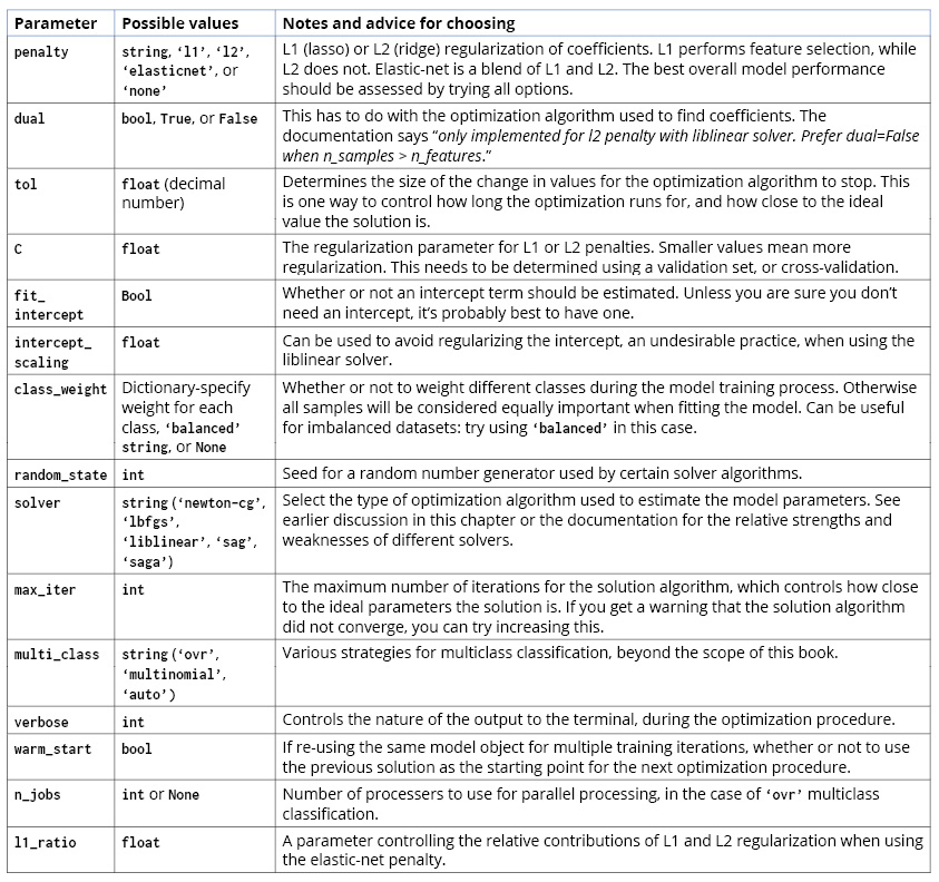
Figure 4.23: A complete list of options for the logistic regression model in scikit-learn
If you are in doubt regarding which option to use for logistic regression, we recommend you consult the scikit-learn documentation for further guidance (https://scikit-learn.org/stable/modules/linear_model.html#logistic-regression). Some options, such as the regularization parameter C, or the choice of a penalty for regularization, will need to be explored through the cross-validation process. Here, as with many choices to be made in data science, there is no universal approach that will apply to all datasets. The best way to see which options to use with a given dataset is to try several of them and see which gives the best out-of-sample performance. Cross-validation offers you a robust way to do this.
Scaling Data, Pipelines, and Interaction Features in Scikit-Learn
Scaling Data
Compared to the synthetic data we were just working with, the case study data is relatively large. If we want to use L1 regularization, then according to the official documentation (https://scikit-learn.org/stable/modules/linear_model.html#logistic-regression), we ought to use the saga solver. However, this solver is not robust to unscaled datasets. Hence, we need to be sure to scale the data. This is also a good idea whenever doing regularization, so all the features are on the same scale and are equally penalized by the regularization process. A simple way to make sure that all the features have the same scale is to put them all through the transformation of subtracting the minimum and dividing by the range from minimum to maximum. This transforms each feature so that it will have a minimum of 0 and a maximum of 1. To instantiate the MinMaxScaler scaler that does this, we can use the following code:
from sklearn.preprocessing import MinMaxScaler
min_max_sc = MinMaxScaler()
Pipelines
Previously, we used a logistic regression model in the cross-validation loop. However, now that we're scaling data, what new considerations are there? The scaling is effectively "learned" from the minimum and maximum values of the training data. After this, a logistic regression model would be trained on data scaled by the extremes of the model training data. However, we won't know the minimum and maximum values of the new, unseen data. So, following the philosophy of making cross-validation an effective indicator of model performance on unseen data, we need to use the minimum and maximum values of the training data in each cross-validation fold in order to scale the test data in that fold, before making predictions on the test data. Scikit-learn has the functionality to facilitate the combination of several training and test steps for situations such as this: the Pipeline. Our pipeline will consist of two steps: the scaler and the logistic regression model. These can both be fit on the training data and then used to make predictions on the test data. The process of fitting a pipeline is executed as a single step in the code, so all the parts of the pipeline are fit at once in this sense. Here is how a Pipeline is instantiated:
from sklearn.pipeline import Pipeline
scale_lr_pipeline = Pipeline(steps=[('scaler', min_max_sc), \
                                    ('model', lr)])
Interaction Features
Considering the case study data, do you think a logistic regression model with all possible features would be overfit or underfit? You can think about this from the perspective of rules of thumb, such as the "rule of 10," and the number of features (17) versus samples (26,664) that we have. Alternatively, you can consider all the work we've done so far with this data. For instance, we've had a chance to visualize all the features and ensure they make sense. Since there are relatively few features, and we have relatively high confidence that they are high quality because of our data exploration work, we are in a different situation than with the synthetic data exercises in this chapter, where we had a large number of features about which we knew relatively little. So, it may be that overfitting will be less of an issue with our case study at this point, and the benefits of regularization may not be significant.
In fact, it may be that we will underfit the model using only the 17 features that came with the data. One strategy to deal with this is to engineer new features. Some simple feature engineering techniques we've discussed include interaction and polynomial features. Polynomials may not make sense given the way in which some of the data has been encoded; for example, -12 = 1, which may not be sensible for PAY_1. However, we may wish to try creating interaction features to capture the relationships between features. PolynomialFeatures can be used to create interaction features only, without polynomial features. The example code is as follows:
make_interactions = PolynomialFeatures(degree=2, \
                                       interaction_only=True, \
                                       include_bias=False)
Here, degree represents the degree of the polynomial features, interaction_only takes a Boolean value (setting it to True indicates that only interaction features will be created), and so does include_bias, which adds an intercept to the model (the default value is False, which is correct here as the logistic regression model will add an intercept).
Activity 4.01: Cross-Validation and Feature Engineering with the Case Study Data
In this activity, we'll apply the knowledge of cross-validation and regularization that we've learned in this chapter to the case study data. We'll perform basic feature engineering. In order to estimate parameters for the regularized logistic regression model for the case study data, which is larger in size than the synthetic data that we've worked with, we'll use the saga solver. In order to use this solver, and for the purpose of regularization, we'll need to scale our data as part of the modeling process, leading us to the use of Pipeline class in scikit-learn. Once you have completed the activity, you should obtain an improved cross-validation test performance with the use of interaction features, as shown in the following diagram:
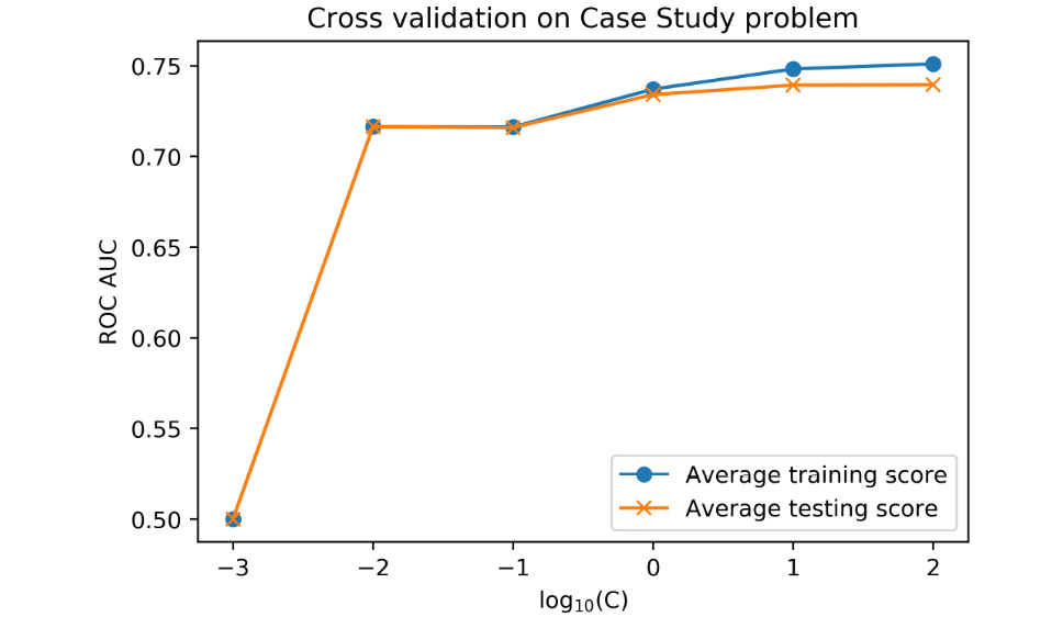
Figure 4.24: Improved model test performance
Perform the following steps to complete the activity:
- Select the features from the DataFrame of the case study data.
You can use the list of feature names that we've already created in this chapter, but be sure not to include the response variable, which would be a very good (but entirely inappropriate) feature!
- Make a training/test split using a random seed of 24.
We'll use this going forward and reserve this test data as the unseen test set. By specifying the random seed, we can easily create separate notebooks with other modeling approaches using the same training data.
- Instantiate
MinMaxScalerto scale the data. - Instantiate a logistic regression model with the
sagasolver, L1 penalty, and setmax_iterto1000as we want the solver to have enough iterations to find a good solution. - Import the
Pipelineclass and create a pipeline with the scaler and the logistic regression model, using the names'scaler'and'model'for the steps, respectively. - Use the
get_paramsandset_paramsmethods to see how to view the parameters from each stage of the pipeline and change them. - Create a smaller range of C values to test with cross-validation, as these models will take longer to train and test with more data than our previous exercise; we recommend C = [102, 10, 1, 10-1, 10-2, 10-3].
- Make a new version of the
cross_val_C_searchfunction calledcross_val_C_search_pipe. Instead of themodelargument, this function will take apipelineargument. The changes inside the function will be to set the C value usingset_params(model__C = <value you want to test>)on the pipeline, replacing the model with the pipeline for thefitandpredict_probamethods, and accessing the C value usingpipeline.get_params()['model__C']for the printed status update. - Run this function as in the previous exercise, but using the new range of C values, the pipeline you created, and the features and response variable from the training split of the case study data.
You may see warnings here, or in later steps, regarding the non-convergence of the solver; you could experiment with the
tolormax_iteroptions to try and achieve convergence, although the results you obtain withmax_iter = 1000are likely to be sufficient. - Plot the average training and test ROC AUC across folds for each C value.
- Create interaction features for the case study data and confirm that the number of new features makes sense.
- Repeat the cross-validation procedure and observe the model performance when using interaction features.
Note that this will take substantially more time, due to the larger number of features, but it will probably take less than 10 minutes. So, does the average cross-validation test performance improve with the interaction features? Is regularization useful?
Note
The Jupyter notebook containing the Python code for this activity can be found at https://packt.link/ohGgX. Detailed step-wise solution to this activity can be found via this link.


