Search icon CANCEL
Subscription
0
Cart icon
Your Cart (0 item)
Close icon
You have no products in your basket yet
Save more on your purchases! discount-offer-chevron-icon
Savings automatically calculated. No voucher code required.
Arrow left icon
Explore Products
Best Sellers
New Releases
Books
Videos
Audiobooks
Learning Hub
Free Learning
Arrow right icon
Arrow up icon
GO TO TOP
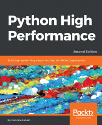
Python High Performance, Second Edition

You're reading from   Python High Performance, Second Edition Build high-performing, concurrent, and distributed applications

Arrow left icon
Product type Paperback
Published in May 2017
Publisher Packt
ISBN-13 9781787282896
Length 270 pages
Edition 2nd Edition
Languages
Tools
Arrow right icon
Author (1):
Arrow left icon
Dr. Gabriele Lanaro Dr. Gabriele Lanaro
Author Profile Icon Dr. Gabriele Lanaro
Dr. Gabriele Lanaro
Arrow right icon
View More author details
Toc

Table of Contents (10) Chapters Close

Preface Benchmarking and Profiling FREE CHAPTER Pure Python Optimizations Fast Array Operations with NumPy and Pandas C Performance with Cython Exploring Compilers Implementing Concurrency Parallel Processing Distributed Processing Designing for High Performance

Writing tests and benchmarks

Now that we have a working simulator, we can start measuring our performance and tune-up our code so that the simulator can handle as many particles as possible. As a first step, we will write a test and a benchmark.

We need a test that checks whether the results produced by the simulation are correct or not. Optimizing a program commonly requires employing multiple strategies; as we rewrite our code multiple times, bugs may easily be introduced. A solid test suite ensures that the implementation is correct at every iteration so that we are free to go wild and try different things with the confidence that, if the test suite passes, the code will still work as expected.

Our test will take three particles, simulate them for 0.1 time units, and compare the results with those from a reference implementation. A good way to organize your tests is using a separate function for each different aspect (or unit) of your application. Since our current functionality is included in the evolve method, our function will be named test_evolve. The following code shows the test_evolve implementation. Note that, in this case, we compare floating point numbers up to a certain precision through the fequal function:

    def test_evolve(): 
particles = [Particle( 0.3, 0.5, +1),
Particle( 0.0, -0.5, -1),
Particle(-0.1, -0.4, +3)]

simulator = ParticleSimulator(particles)

simulator.evolve(0.1)

p0, p1, p2 = particles

def fequal(a, b, eps=1e-5):
return abs(a - b) < eps

assert fequal(p0.x, 0.210269)
assert fequal(p0.y, 0.543863)

assert fequal(p1.x, -0.099334)
assert fequal(p1.y, -0.490034)

assert fequal(p2.x, 0.191358)
assert fequal(p2.y, -0.365227)

if __name__ == '__main__':
test_evolve()

A test ensures the correctness of our functionality but gives little information about its running time. A benchmark is a simple and representative use case that can be run to assess the running time of an application. Benchmarks are very useful to keep score of how fast our program is with each new version that we implement.

We can write a representative benchmark by instantiating a thousand Particle objects with random coordinates and angular velocity, and feed them to a ParticleSimulator class. We then let the system evolve for 0.1 time units:

    from random import uniform 

def benchmark():
particles = [Particle(uniform(-1.0, 1.0),
uniform(-1.0, 1.0),
uniform(-1.0, 1.0))
for i in range(1000)]

simulator = ParticleSimulator(particles)
simulator.evolve(0.1)

if __name__ == '__main__':
benchmark()

Timing your benchmark

A very simple way to time a benchmark is through the Unix time command. Using the time command, as follows, you can easily measure the execution time of an arbitrary process:

    $ time python simul.py
real 0m1.051s
user 0m1.022s
sys 0m0.028s
The time command is not available for Windows. To install Unix tools, such as time, on Windows you can use the cygwin shell, downloadable from the official website (http://www.cygwin.com/). Alternatively, you can use similar PowerShell commands, such as Measure-Command (https://msdn.microsoft.com/en-us/powershell/reference/5.1/microsoft.powershell.utility/measure-command), to measure execution time.

By default, time displays three metrics:

  • real: The actual time spent running the process from start to finish, as if it was measured by a human with a stopwatch
  • user: The cumulative time spent by all the CPUs during the computation
  • sys: The cumulative time spent by all the CPUs during system-related tasks, such as memory allocation

Note that sometimes user + sys might be greater than real, as multiple processors may work in parallel.

time also offers richer formatting options. For an overview, you can explore its manual (using the man time command). If you want a summary of all the metrics available, you can use the -v option.

The Unix time command is one of the simplest and more direct ways to benchmark a program. For an accurate measurement, the benchmark should be designed to have a long enough execution time (in the order of seconds) so that the setup and tear-down of the process is small compared to the execution time of the application. The user metric is suitable as a monitor for the CPU performance, while the real metric also includes the time spent in other processes while waiting for I/O operations.

Another convenient way to time Python scripts is the timeit module. This module runs a snippet of code in a loop for n times and measures the total execution times. Then, it repeats the same operation r times (by default, the value of r is 3) and records the time of the best run. Due to this timing scheme, timeit is an appropriate tool to accurately time small statements in isolation.

The timeit module can be used as a Python package, from the command line or from IPython.

IPython is a Python shell design that improves the interactivity of the Python interpreter. It boosts tab completion and many utilities to time, profile, and debug your code. We will use this shell to try out snippets throughout the book. The IPython shell accepts magic commands--statements that start with a % symbol--that enhance the shell with special behaviors. Commands that start with %% are called cell magics, which can be applied on multi-line snippets (termed as cells).

IPython is available on most Linux distributions through pip and is included in Anaconda.

You can use IPython as a regular Python shell (ipython), but it is also available in a Qt-based version (ipython qtconsole) and as a powerful browser-based interface (jupyter notebook).

In IPython and command-line interfaces, it is possible to specify the number of loops or repetitions with the -n and -r options. If not specified, they will be automatically inferred by timeit. When invoking timeit from the command line, you can also pass some setup code, through the -s option, which will execute before the benchmark. In the following snippet, the IPython command line and Python module version of timeit are demonstrated:

# IPython Interface 
$ ipython
In [1]: from simul import benchmark
In [2]: %timeit benchmark()
1 loops, best of 3: 782 ms per loop

# Command Line Interface
$ python -m timeit -s 'from simul import benchmark' 'benchmark()'
10 loops, best of 3: 826 msec per loop

# Python Interface
# put this function into the simul.py script

import timeit
result = timeit.timeit('benchmark()',
setup='from __main__ import benchmark',
number=10)

# result is the time (in seconds) to run the whole loop
result = timeit.repeat('benchmark()',
setup='from __main__ import benchmark',
number=10,
repeat=3)
# result is a list containing the time of each repetition (repeat=3 in this case)

Note that while the command line and IPython interfaces automatically infer a reasonable number of loops n, the Python interface requires you to explicitly specify a value through the number argument.

You have been reading a chapter from
Python High Performance, Second Edition - Second Edition
Published in: May 2017
Publisher: Packt
ISBN-13: 9781787282896
Register for a free Packt account to unlock a world of extra content!
A free Packt account unlocks extra newsletters, articles, discounted offers, and much more. Start advancing your knowledge today.
Unlock this book and the full library FREE for 7 days
Get unlimited access to 7000+ expert-authored eBooks and videos courses covering every tech area you can think of
Renews at $19.99/month. Cancel anytime
Banner background image