Building a transformer model for language modeling

In this section, we will explore what transformers are and build one using PyTorch for the task of language modeling. We will also learn how to use some advanced transformer-based models, such as BERT and GPT, via PyTorch’s pretrained model repository. The pretrained model repository contains PyTorch models trained on general tasks such as language modeling (predicting the next word given the sequence of preceding words). These pretrained models can then be fine-tuned for specific tasks such as sentiment analysis (whether a given piece of writing is positive, negative or neutral). Before we start building a transformer model, let’s quickly recap what language modeling is.

Reviewing language modeling

Language modeling is the task of figuring out the probability of the occurrence of a word or a sequence of words that should follow a given sequence of words. For example, if we are given French is a beautiful _____ as our sequence of words, what is the probability that the next word will be language or word, and so on? These probabilities are computed by modeling the language using various probabilistic and statistical techniques. The idea is to observe a text corpus and learn the grammar by learning which words occur together and which words never occur together. This way, a language model establishes probabilistic rules around the occurrence of different words or sequences, given various different sequences.

Recurrent models have been a popular way of learning a language model. However, as with many sequence-related tasks, transformers have outperformed recurrent networks on this task as well. We will implement a transformer-based language model for the English language by training it on a text corpus based on articles from the Wall Street Journal.

Now, let’s start training a transformer for language modeling. During this exercise, we will demonstrate only the most important parts of the code. The full code can be accessed in our GitHub repository [1].

We will delve deeper into the various components of the transformer architecture in-between the exercise.

For this exercise, we will need to import a few dependencies. One of the important import statements is listed here:

from torch.nn import TransformerEncoder, TransformerEncoderLayer

Besides importing the regular torch dependencies, we must import some modules specific to the transformer model; these are provided directly under the torch library. We’ll also import torchtext in order to download a text dataset directly from the available datasets under torchtext.datasets.

In the next section, we will define the transformer model architecture and look at the details of the model’s components.

Understanding the transformer model architecture

This is perhaps the most important step of this exercise. Here, we define the architecture of the transformer model.

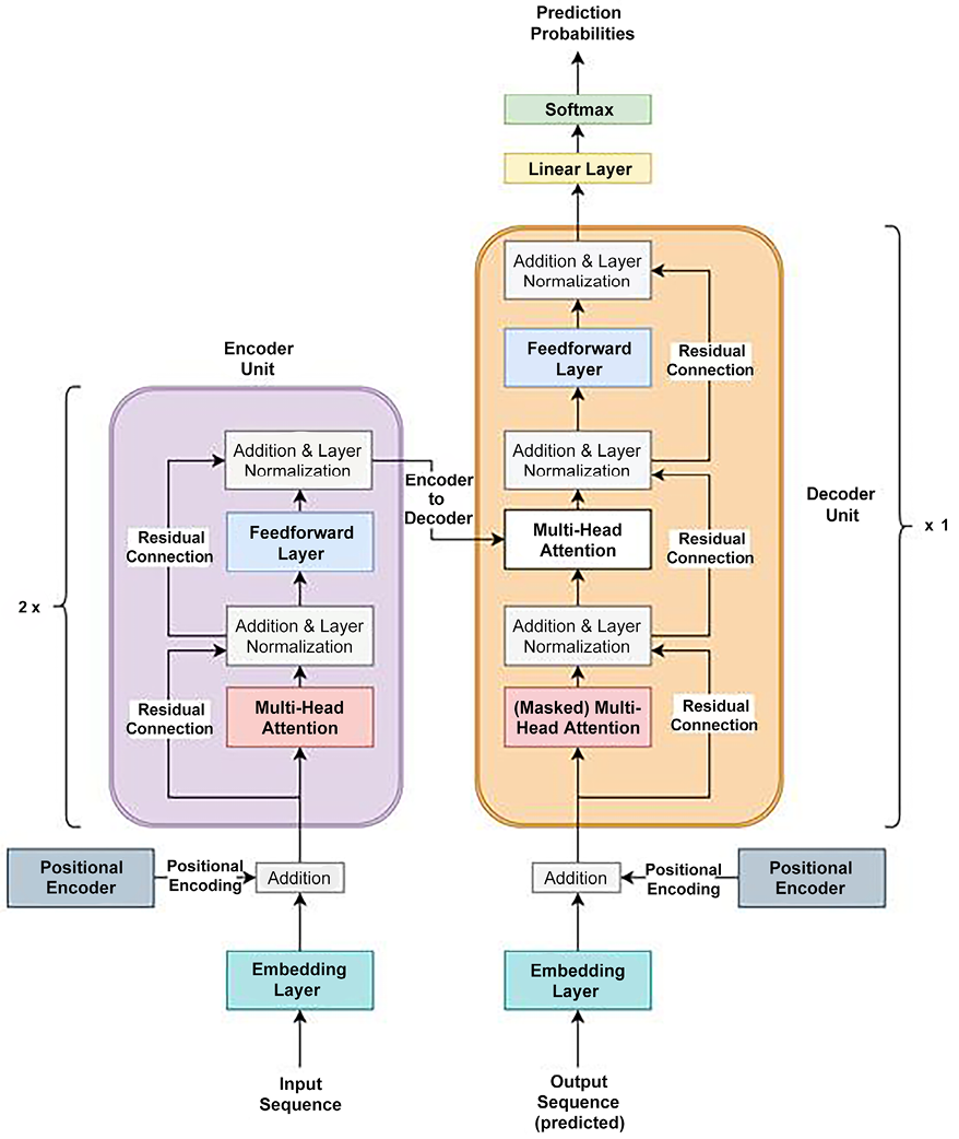
First, let’s briefly discuss the model architecture and then look at the PyTorch code for defining the model. Figure 5.1 shows the model architecture:

Figure 5.1: Transformer model architecture

The first thing to notice is that this is essentially an encoder-decoder-based architecture, with the Encoder Unit on the left (in purple) and the Decoder Unit (in orange) on the right. The encoder and decoder units can be tiled multiple times for even deeper architectures. In our example, we have two cascaded encoder units and a single decoder unit. This encoder-decoder setup essentially means that the encoder takes a sequence as input and generates as many embeddings as there are words in the input sequence (that is, one embedding per word). These embeddings are then fed to the decoder, along with the predictions made thus far by the model.

Let’s walk through the various layers in this model:

• Embedding Layer: This layer is simply meant to perform the traditional task of converting each input word of the sequence into a vector of numbers – that is, an embedding. As always, here, we use the torch.nn.Embedding module to code this layer.
• Positional Encoder: Note that transformers do not have any recurrent layers in their architecture, yet they outperform recurrent networks on sequential tasks. How? Using a neat trick known as positional encoding, the model is provided a sense of sequentiality or sequential-order in the data. Basically, vectors that follow a particular sequential pattern are added to the input word embeddings.

These vectors are generated in a way that enables the model to understand that the second word comes after the first word and so on. The vectors are generated using the sinusoidal and cosinusoidal functions to represent a systematic periodicity and distance between subsequent words, respectively. The implementation of this layer for our exercise is as follows:

class PosEnc(nn.Module):
    def __init__(self, d_m, dropout=0.2, size_limit=5000):
        # d_m is same as the dimension of the embeddings
        pos = torch.arange(size_limit, dtype=torch.float).unsqueeze(1)
        divider = torch.exp(
            torch.arange(0, d_m, 2).float() * (
                -torch.log(10000.0) / d_m))
        '''divider is the list of radians, multiplied by 
           position indices of words, and fed to the 
           sinusoidal and cosinusoidal function.'''
        p_enc[:, 0, 0::2] = torch.sin(pos * divider)
        p_enc[:, 0, 1::2] = torch.cos(pos * divider)
    def forward(self, x):
        return self.dropout(x + self.p_enc[:x.size(0)])

As you can see, the sinusoidal and cosinusoidal functions are used alternately to give the sequential pattern. There are many ways to implement positional encoding though. Without a positional encoding layer, the model will be clueless about the order of the words.

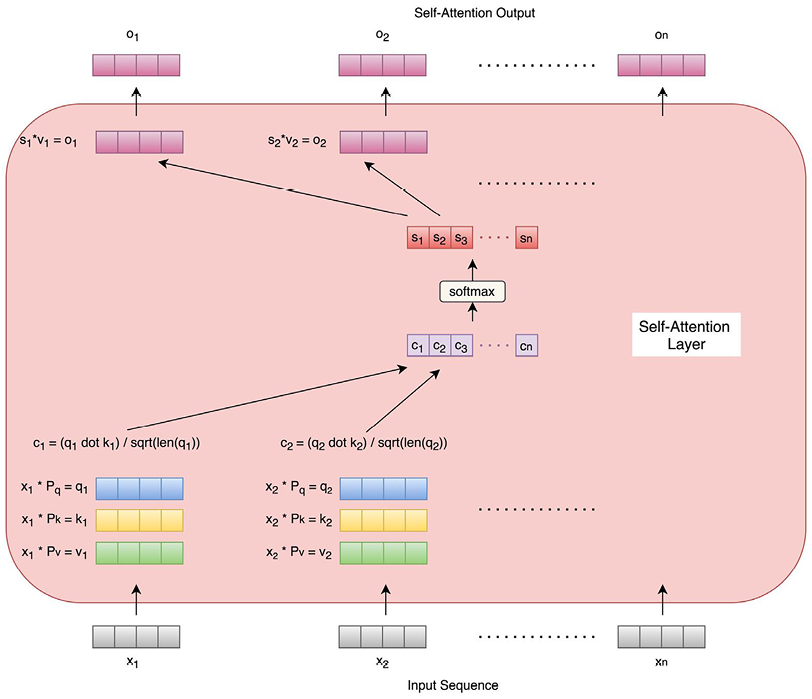
• Multi-Head Attention: Before we look at the multi-head attention layer, let’s first understand what a self-attention layer is. We covered the concept of attention in Chapter 4, Deep Recurrent Model Architectures, with respect to recurrent networks. Here, as the name suggests, the attention mechanism is applied to self – that is, each word of the sequence. Each word embedding of the sequence goes through the self-attention layer and produces an individual output that is exactly the same length as the word embedding. Figure 5.2 describes the process of this in detail:

Figure 5.2: Self-attention layer

As we can see, for each word, three vectors are generated through three learnable parameter matrices (P_q, P_k, and P_v). The three vectors are query, key, and value vectors. The query and key vectors are dot-multiplied to produce a number for each word. These numbers are normalized by dividing the square root of the key vector length for each word. The resultant numbers for all words are then Softmaxed at the same time to produce probabilities that are finally multiplied by the respective value vectors for each word. This results in one output vector for each word of the sequence, with the lengths of the output vector and the input word embedding being the same.

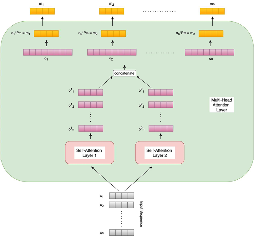
A multi-head attention layer is an extension of the self-attention layer where multiple self-attention modules compute outputs for each word. These individual outputs are concatenated and matrix-multiplied with yet another parameter matrix (P_m) to generate the final output vector, whose length is equal to the input embedding vector’s. The following diagram shows the multi-head attention layer, along with two self-attention units that we will be using in this exercise:

Figure 5.3: Multi-head attention layer with two self-attention units

Having multiple self-attention heads helps different heads focus on different aspects of the sequence of words, similar to how different feature maps learn different patterns in a convolutional neural network. Due to this, the multi-head attention layer performs better than an individual self-attention layer and will be used in our exercise.

Also, note that the masked multi-head attention layer in the decoder unit works in exactly the same way as a multi-head attention layer, except for the added masking – that is, given the time step t of processing the sequence, all words from t+1 to n (the length of the sequence) are masked/hidden.

During training, the decoder is provided with two types of inputs. On one hand, it receives query and key vectors from the final encoder as inputs to its (unmasked) multi-head attention layer, where these query and key vectors are matrix transformations of the final encoder output. On the other hand, the decoder receives its own predictions from previous time steps as sequential input to its masked multi-head attention layer.

• Addition and Layer Normalization: We discussed the concept of a residual connection in Chapter 2, Deep CNN Architectures, while discussing ResNets. In Figure 5.1, we can see that there are residual connections across the addition and layer normalization layers. In each instance, a residual connection is established by directly adding the input word-embedding vector to the output vector of the multi-head attention layer. This helps with easier gradient flow throughout the network and avoids problems with exploding and vanishing gradients. Also, it helps with efficiently learning identity functions across layers.

Furthermore, layer normalization is used as a normalization trick. Here, we normalize each feature independently so that all the features have a uniform mean and standard deviation. Please note that these additions and normalizations are applied individually to each word vector of the sequence at each stage of the network.

• Feedforward Layer: Within both the encoder and decoder units, the normalized residual output vectors for all the words of the sequence are passed through a common feedforward layer. Due to there being a common set of parameters across words, this layer helps with learning broader patterns across the sequence.
• Linear and Softmax Layer: So far, each layer is outputting a sequence of vectors, one per word. For our task of language modeling, we need a single final output. The linear layer transforms the sequence of vectors into a single vector whose size is equal to the length of our word vocabulary. The Softmax layer converts this output into a vector of probabilities summing to 1. These probabilities are the probabilities that the respective words (in the vocabulary) occur as the next words in the sequence.

Now that we have elaborated on the various elements of a transformer model, let’s look at the PyTorch code to instantiate the model.

Defining a transformer model in PyTorch

Using the architecture details described in the previous section, we will now write the necessary PyTorch code to define a transformer model, as follows:

class Transformer(nn.Module):
    def __init__(self, num_token, num_inputs, num_heads, num_hidden,
                 num_layers, dropout=0.3):
        self.position_enc = PosEnc(num_inputs, dropout)
        layers_enc = TransformerEncoderLayer(
            num_inputs, num_heads, num_hidden, dropout)
        self.enc_transformer = TransformerEncoder(
            layers_enc, num_layers)
        self.enc = nn.Embedding(num_token, num_inputs)
        self.num_inputs = num_inputs
        self.dec = nn.Linear(num_inputs, num_token)

As we can see, in the __init__ method of the class, thanks to PyTorch’s TransformerEncoder and TransformerEncoderLayer functions, we do not need to implement these ourselves. For our language modeling task, we just need a single output for the input sequence of words. Due to this, the decoder is just a linear layer that transforms the sequence of vectors from an encoder into a single output vector. A position encoder is also initialized using the definition that we discussed earlier.

In the forward method, the input is positionally encoded and then passed through the encoder, followed by the decoder:

    def forward(self, source):
        source = self.enc(source) * torch.sqrt(self.num_inputs)
        source = self.position_enc(source)
        op = self.enc_transformer(source, self.mask_source)
        op = self.dec(op)
        return op

Now that we have defined the transformer model architecture, we shall load the text corpus to train it on.

Loading and processing the dataset

In this section, we will discuss the steps related to loading a text dataset for our task and making it usable for the model training routine. Let’s get started:

1. For this exercise, we will be using texts from the Wall Street Journal, available as the Penn Treebank dataset.

Dataset citation

Marcus Mitchell P., Marcinkiewicz Mary Ann, and Santorini Beatrice. 1993. Building a large annotated corpus of english: The Penn Treebank: https://github.com/wojzaremba/lstm/tree/master/data

We’ll use the functionality of torchtext to download the training dataset (available under the torchtext datasets) and tokenize its vocabulary:

tr_iter = PennTreebank(split='train')
tkzer = get_tokenizer('basic_english')
vocabulary = build_vocab_from_iterator(
    map(tkzer, tr_iter), specials=['<unk>'])
vocabulary.set_default_index(vocabulary['<unk>'])

2. We will then use the vocabulary to convert raw text into tensors for the training, validation, and testing datasets:

   def process_data(raw_text):
       numericalised_text = [
           torch.tensor(vocabulary(tkzer(text)),
                        dtype=torch.long) for text in raw_text]
       return torch.cat(
           tuple(filter(lambda t: t.numel() > 0,
                        numericalised_text)))
   tr_iter, val_iter, te_iter = PennTreebank()
   training_text = process_data(tr_iter)
   validation_text = process_data(val_iter)
   testing_text = process_data(te_iter)
   

3. We’ll also define the batch sizes for training and evaluation and declare a batch generation function, as shown here:

   def gen_batches(text_dataset, batch_size):
       num_batches = text_dataset.size(0) // batch_size
       text_dataset = text_dataset[:num_batches * batch_size]
       text_dataset = text_dataset.view(
           batch_size, num_batches).t().contiguous()
       return text_dataset.to(device)
   training_batch_size = 32
   evaluation_batch_size = 16
   training_data = gen_batches(training_text, training_batch_size)
   

4. Next, we must define the maximum sequence length and write a function that will generate input sequences and output targets for each batch, accordingly:

   max_seq_len = 64
   def return_batch(src, k):
       sequence_length = min(max_seq_len, len(src) - 1 - k)
       sequence_data = src[k:k+sequence_length]
       sequence_label = src[k+1:k+1+sequence_length].reshape(-1)
       return sequence_data, sequence_label
   

Having defined the model and prepared the training data, we will now train the transformer model.

Training the transformer model

In this section, we will define the necessary hyperparameters for model training, define the model training and evaluation routines, and finally, execute the training loop. Let’s get started:

1. In this step, we define all the model hyperparameters and instantiate our transformer model. The following code is self-explanatory:

   num_tokens = len(vocabulary) # vocabulary size
   embedding_size = 256 # dimension of embedding layer
   # transformer encoder's hidden (feed forward) layer dimension
   num_hidden_params = 256
   # num of transformer encoder layers within transformer encoder
   num_layers = 2
   # num of heads in (multi head) attention models
   num_heads = 2
   # value (fraction) of dropout
   dropout = 0.25
   loss_func = nn.CrossEntropyLoss()
   # learning rate
   lrate = 4.0
   optim_module = torch.optim.SGD(transformer_model.parameters(), lr=lrate)
   sched_module = torch.optim.lr_scheduler.StepLR(
       optim_module, 1.0, gamma=0.88)
   transformer_model = Transformer(
       num_tokens, embedding_size, num_heads,
       num_hidden_params, num_layers, dropout).to(device)
   

2. Before starting the model training and evaluation loop, we need to define the training and evaluation routines:

   def train_model():
       for b, i in enumerate(
           range(0, training_data.size(0) - 1, max_seq_len)):
           train_data_batch, train_label_batch = return_batch(
               training_data, i)
           sequence_length = train_data_batch.size(0)
           # only on last batch
           if sequence_length != max_seq_len:
               mask_source = mask_source[:sequence_length,
                                         :sequence_length]
           op = transformer_model(train_data_batch, mask_source)
           loss_curr = loss_func(op.view(-1, num_tokens), train_label_batch)
           optim_module.zero_grad()
           loss_curr.backward()
   torch.nn.utils.clip_grad_norm_(transformer_model.parameters(), 0.6)
   optim_module.step()
   loss_total += loss_curr.item()
   def eval_model(eval_model_obj, eval_data_source):
   ...
   

3. Finally, we must run the model training loop. For demonstration purposes, we are training the model for 5 epochs, but you are encouraged to run it for longer in order to get better performance:

   min_validation_loss = float("inf")
   eps = 5
   best_model_so_far = None
   for ep in range(1, eps + 1):
       ep_time_start = time.time()
       train_model()
       validation_loss = eval_model(transformer_model, validation_data)
       if validation_loss < min_validation_loss:
           min_validation_loss = validation_loss
           best_model_so_far = transformer_model
   

This should result in the following output:

epoch 1, 100/1000 batches, training loss 8.77, training perplexity 6460.73
epoch 1, 200/1000 batches, training loss 7.30, training perplexity 1480.28
epoch 1, 300/1000 batches, training loss 6.88, training perplexity 969.18
...
epoch 5, 900/1000 batches, training loss 5.19, training perplexity 178.59
epoch 5, 1000/1000 batches, training loss 5.27, training perplexity 193.60
epoch 5, validation loss 5.32, validation perplexity 204.29

Besides the cross-entropy loss, the perplexity is also reported. Perplexity is a popularly used metric in natural language processing to indicate how well a probability distribution (a language model, in our case) fits or predicts a sample. The lower the perplexity, the better the model is at predicting the sample. Mathematically, perplexity is just the exponential of the cross-entropy loss. Intuitively, this metric is used to indicate how perplexed or confused the model is while making predictions.

4. Once the model has been trained, we can conclude this exercise by evaluating the model’s performance on the test set:

   testing_loss = eval_model(best_model_so_far, testing_data)
   print(f"testing loss {testing_loss:.2f}, testing perplexity {math.exp(testing_loss):.2f}")
   

This should result in the following output:

testing loss 5.23, testing perplexity 187.45

In this exercise, we built a transformer model using PyTorch for the task of language modeling. We explored the transformer architecture in detail and how it is implemented in PyTorch. We used the Penn Treebank dataset and torchtext functionalities to load and process the dataset. We then trained the transformer model for 5 epochs and evaluated it on a separate test set. This shall provide us with all the information we need to get started on working with transformers.

Besides the original transformer model, which was devised in 2017, a number of successors have since been developed over the years, especially around the field of language modeling, such as the following:

• Bidirectional Encoder Representations from Transformers (BERT), 2018
• Generative Pretrained Transformer (GPT), 2018
• GPT-2, 2019
• Conditional Transformer Language Model (CTRL), 2019
• Transformer-XL, 2019
• Distilled BERT (DistilBERT), 2019
• Robustly optimized BERT pretraining Approach (RoBERTa), 2019
• GPT-3, 2020
• Text-To-Text-Transfer-Transformer (T5), 2020
• Language Model for Dialogue Operations (LaMDA), 2021
• Pathways Language Model (PaLM), 2022
• GPT-3.5 (ChatGPT), 2022
• Large Language Model Meta AI (LLaMA), 2023
• GPT-4, 2023
• LLaMA-2, 2023
• Grok, 2023
• Gemini, 2023
• Sora, 2024
• Gemini-1.5, 2024
• LLaMA-3, 2024

While we will not cover these models in detail in this chapter, you can nonetheless get started using these models with PyTorch thanks to the transformers library, developed by Hugging Face [2]. We will explore Hugging Face in detail in Chapter 19, PyTorch x Hugging Face. The transformers library provides pretrained transformer models for various tasks, such as language modeling, text classification, translation, question-answering, and so on.

Besides the models themselves, it also provides tokenizers for the respective models. For example, if we wanted to use a pretrained BERT model for language modeling, we would need to write the following code once we have installed the transformers library:

import torch
from transformers import BertForMaskedLM, BertTokenizer
bert_model = BertForMaskedLM.from_pretrained('bert-base-uncased')
token_gen = BertTokenizer.from_pretrained('bert-base-uncased')
ip_sequence = token_gen("I love PyTorch !", return_tensors="pt")["input_ids"]
op = bert_model(ip_sequence, labels=ip_sequence)
total_loss, raw_preds = op[:2]

As we can see, it takes just a couple of lines to get started with a BERT-based language model. This demonstrates the power of the PyTorch ecosystem. You are encouraged to explore this with more complex variants, such as DistilBERT or RoBERTa, using the transformers library. For more details, please refer to their GitHub page, which was mentioned previously.

This concludes our exploration of transformers. We did this by both building one from scratch as well as by reusing pretrained models. The invention of transformers in the natural language processing space has a parallel with the ImageNet moment in the field of computer vision, so this is going to be an active area of research. PyTorch will have a crucial role to play in the research and deployment of these types of models.

In the next and final section of this chapter, we will resume the neural architecture search discussions we provided at the end of Chapter 2, Deep CNN Architectures, where we briefly discussed the idea of generating optimal network architectures. We will explore a type of model where we do not decide what the model architecture will look like, and instead run a network generator that will find an optimal architecture for the given task. The resultant network is called a randomly wired neural network (RandWireNN), and we will develop one from scratch using PyTorch.