Most popular LLM transformers-based architectures
ANNs, as we saw in the preceding sections, are at the heart of LLMs. Nevertheless, in order to be generative, those ANNs need to be endowed with some peculiar capabilities, such as parallel processing of textual sentences or keeping the memory of the previous context.
These particular capabilities were at the core of generative AI research in the last decades, starting from the 80s and 90s. However, it is only in recent years that the main drawbacks of these early models – such as the capability of text parallel processing or memory management – have been bypassed by modern generative AI frameworks. Those frameworks are the so-called transformers.
In the following sections, we will explore the evolution of generative AI model architecture, from early developments to state-of-the-art transformers. We will start by covering the first generative AI models that paved the way for further research, highlighting their limitations and the approaches to overcome them. We will then explore the introduction of transformer-based architectures, covering their main components and explaining why they represent the state of the art for LLMs.
Early experiments
The very first popular generative AI ANN architectures trace back to the 80s and 90s, including:
- Recurrent neural networks (RNNs): RNNs are a type of ANN designed to handle sequential data. They have recurrent connections that allow information to persist across time steps, making them suitable for tasks like language modeling, machine translation, and text generation. However, RNNs have limitations in capturing long-range dependencies due to the vanishing or exploding gradient problem.
Definition
In ANNs, the gradient is a measure of how much the model’s performance would improve if we slightly adjusted its internal parameters (weights). During training, RNNs try to minimize the difference between their predictions and the actual targets by adjusting their weights based on the gradient of the loss function. The problem of vanishing or exploding gradient arises in RNNs during training when the gradients become extremely small or large, respectively. The vanishing gradient problem occurs when the gradient becomes extremely small during training. As a result, the RNN learns very slowly and struggles to capture long-term patterns in the data. Conversely, the exploding gradient problem happens when the gradient becomes extremely large. This leads to unstable training and prevents the RNN from converging to a good solution.
- Long short-term memory (LSTM): LSTMs are a variant of RNNs that address the vanishing gradient problem. They introduce gating mechanisms that enable better preservation of important information across longer sequences. LSTMs became popular for various sequential tasks, including text generation, speech recognition, and sentiment analysis.
These architectures were popular and effective for various generative tasks, but they had limitations in handling long-range dependencies, scalability, and overall efficiency, especially when dealing with large-scale NLP tasks that would need massive parallel processing. The transformer framework was introduced to overcome these limitations. In the next section, we are going to see how a transformers-based architecture overcomes the above limitations and is at the core of modern generative AI LLMs.
Introducing the transformer architecture
The transformer architecture is a deep learning model introduced in the paper “Attention Is All You Need” by Vaswani et al. (2017). It revolutionized NLP and other sequence-to-sequence tasks.
The transformer dispenses with recurrence and convolutions entirely and relies solely on attention mechanisms to encode and decode sequences.
Definition
In the transformer architecture, “attention” is a mechanism that enables the model to focus on relevant parts of the input sequence while generating the output. It calculates attention scores between input and output positions, applies Softmax to get weights, and takes a weighted sum of the input sequence to obtain context vectors. Attention is crucial for capturing long-range dependencies and relationships between words in the data.
Since transformers use attention on the same sequence that is currently being encoded, we refer to it as self-attention. Self-attention layers are responsible for determining the importance of each input token in generating the output. Those answer the question: “Which part of the input should I focus on?”
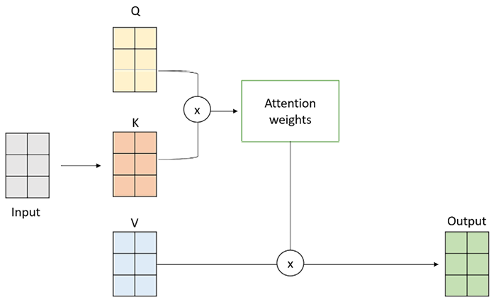
In order to obtain the self-attention vector for a sentence, the elements we need are “value”, “query”, and “key.” These matrices are used to calculate attention scores between the elements in the input sequence and are the three weight matrices that are learned during the training process (typically initialized with random values). More specifically, their purpose is as follows:
- Query (Q) is used to represent the current focus of the attention mechanism
- Key (K) is used to determine which parts of the input should be given attention
- Value (V) is used to compute the context vectors
They can be represented as follows:

Figure 1.8: Decomposition of the Input matrix into Q, K, and V vectors
Those matrices are then multiplied and passed through a non-linear transformation (thanks to a Softmax function). The output of the self-attention layer represents the input values in a transformed, context-aware manner, which allows the transformer to attend to different parts of the input depending on the task at hand.

Figure 1.9: Representation of Q, K, and V matrices multiplication to obtain the context vector
The mathematical formula is the following:

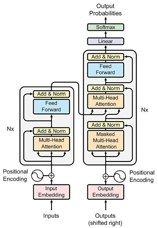
From an architectural point of view, the transformer consists of two main components, an encoder and a decoder:
- The encoder takes the input sequence and produces a sequence of hidden states, each of which is a weighted sum of all the input embeddings.
- The decoder takes the output sequence (shifted right by one position) and produces a sequence of predictions, each of which is a weighted sum of all the encoder’s hidden states and the previous decoder’s hidden states.
Note
The reason for shifting the output sequence right by one position in the decoder layer is to prevent the model from seeing the current token when predicting the next token. This is because the model is trained to generate the output sequence given the input sequence, and the output sequence should not depend on itself. By shifting the output sequence right, the model only sees the previous tokens as input and learns to predict the next token based on the input sequence and the previous output tokens. This way, the model can learn to generate coherent and meaningful sentences without cheating.
The following illustration from the original paper shows the transformer architecture:

Figure 1.10: Simplified transformer architecture
Let’s examine each building block, starting from the encoding part:
- Input embedding: These are the vector representations of tokenized input text.
- Positional encoding: As the transformer does not have an inherent sense of word order (unlike RNNs with their sequential nature), positional encodings are added to the input embeddings. These encodings provide information about the positions of words in the input sequence, allowing the model to understand the order of tokens.
- Multi-head attention layer: This is a mechanism in which multiple self-attention mechanisms operate in parallel on different parts of the input data, producing multiple representations. This allows the transformer model to attend to different parts of the input data in parallel and aggregate information from multiple perspectives.
- Add and norm layer: This combines element-wise addition and layer normalization. It adds the output of a layer to the original input and then applies layer normalization to stabilize and accelerate training. This technique helps mitigate gradient-related issues and improves the model’s performance on sequential data.
- Feed-forward layer: This is responsible for transforming the normalized output of attention layers into a suitable representation for the final output, using a non-linear activation function, such as the previously mentioned Softmax.
The decoding part of the transformer starts with a similar process as the encoding part, where the target sequence (output sequence) undergoes input embedding and positional encoding. Let’s understand these blocks:
- Output embedding (shifted right): For the decoder, the target sequence is “shifted right” by one position. This means that at each position, the model tries to predict the token that comes after the analyzed token in the original target sequence. This is achieved by removing the last token from the target sequence and padding it with a special start-of-sequence token (start symbol). This way, the decoder learns to generate the correct token based on the preceding context during autoregressive decoding.
Definition
Autoregressive decoding is a technique for generating output sequences from a model that predicts each output token based on the previous output tokens. It is often used in NLP tasks such as machine translation, text summarization, and text generation.
Autoregressive decoding works by feeding the model an initial token, such as a start-of-sequence symbol, and then using the model’s prediction as the next input token. This process is repeated until the model generates an end-of-sequence symbol or reaches a maximum length. The output sequence is then the concatenation of all the predicted tokens.
- Decoder layers: Similarly to the encoder block, here, we also have Positional Encoding, Multi-Head Attention, Add and Norm, and Feed Forward layers, whose role is the same as for the encoding part.
- Linear and Softmax: These layers apply, respectively, a linear and non-linear transformation to the output vector. The non-linear transformation (Softmax) conveys the output vector into a probability distribution, corresponding to a set of candidate words. The word corresponding to the greatest element of the probability vector will be the output of the whole process.
The transformer architecture paved the way for modern LLMs, and it also saw many variations with respect to its original framework.
Some models use only the encoder part, such as BERT (Bidirectional Encoder Representations from Transformers), which is designed for NLU tasks such as text classification, question answering, and sentiment analysis.
Other models use only the decoder part, such as GPT-3 (Generative Pre-trained Transformer 3), which is designed for natural language generation tasks such as text completion, summarization, and dialogue.
Finally, there are models that use both the encoder and the decoder parts, such as T5 (Text-to-Text Transfer Transformer), which is designed for various NLP tasks that can be framed as text-to-text transformations, such as translation, paraphrasing, and text simplification.
Regardless of the variant, the core component of a transformer – the attention mechanism – remains a constant within LLM architecture, and it also represents the reason why those frameworks gained so much popularity within the context of generative AI and NLP.
However, the architectural variant of an LLM is not the only element that features the functioning of that model. This functioning is indeed characterized also by what the model knows, depending on its training dataset, and how well it applies its knowledge upon the user’s request, depending on its evaluation metrics.
In the next section, we are going to cover both the processes of training and evaluating LLMs, also providing those metrics needed to differentiate among different LLMs and understand which one to use for specific use cases within your applications.


