Conducting Regression Analysis Using Python
Having discussed the basics of regression analysis, it is now time to get our hands dirty and actually do some regression analysis using Python.
To begin with our analysis, we need to start a session in Python and load the relevant modules and dataset required.
All of the regression analysis we will do in this chapter will be based on the Boston Housing dataset. The dataset is good for teaching and is suitable for linear regression analysis. It presents the level of challenge that necessitates the use of the logarithm function to transform variables in order to achieve a better level of model fit to the data. The dataset contains information on a collection of properties in the Boston area and can be used to determine how the different housing attributes of a specific property affect the property's value.
The column headings of the Boston Housing dataset CSV file can be explained as follows:
- CRIM – per capita crime rate by town
- ZN – proportion of residential land zoned for lots over 25,000 sq.ft.
- INDUS – proportion of non-retail business acres per town
- CHAS – Charles River dummy variable (= 1 if tract bounds river; 0 otherwise)
- NOX – nitric oxide concentration (parts per 10 million)
- RM – average number of rooms per dwelling
- AGE – proportion of owner-occupied units built prior to 1940
- DIS – weighted distances to five Boston employment centers
- RAD – index of accessibility to radial highways
- TAX – full-value property-tax rate per $10,000
- PTRATIO – pupil-teacher ratio by town
- LSTAT – % of lower status of the population
- MEDV – median value of owner-occupied homes in $1,000s
The dataset we're using is a slightly modified version of the original and was sourced from https://packt.live/39IN8Y6.
Exercise 2.01: Loading and Preparing the Data for Analysis
In this exercise, we will learn how to load Python modules, and the dataset we need for analysis, into our Python session and prepare the data for analysis.
Note
We will be using the Boston Housing dataset in this chapter, which can be found on our GitHub repository at https://packt.live/2QCCbQB.
The following steps will help you to complete this exercise:
- Open a new Colab notebook file.
- Load the necessary Python modules by entering the following code snippet into a single Colab notebook cell. Press the Shift and Enter keys together to run the block of code:
%matplotlib inline
import matplotlib as mpl
import seaborn as sns
import matplotlib.pyplot as plt
import statsmodels.formula.api as smf
import statsmodels.graphics.api as smg
import pandas as pd
import numpy as np
import patsy
from statsmodels.graphics.correlation import plot_corr
from sklearn.model_selection import train_test_split
plt.style.use('seaborn')
The first line of the preceding code enables
matplotlibto display the graphical output of the code in the notebook environment. The lines of code that follow use theimportkeyword to load various Python modules into our programming environment. This includespatsy, which is a Python module. Some of the modules are given aliases for easy referencing, such as theseabornmodule being given the aliassns. Therefore, whenever we refer toseabornin subsequent code, we use the aliassns. Thepatsymodule is imported without an alias. We, therefore, use the full name of thepatsymodule in our code where needed.The
plot_corrandtrain_test_splitfunctions are imported from thestatsmodels.graphics.correlationandsklearn.model_selectionmodules respectively. The last statement is used to set the aesthetic look of the graphs thatmatplotlibgenerates to the type displayed by theseabornmodule. - Next, load the
Boston.CSVfile and assign the variable namerawBostonDatato it by running the following code:rawBostonData = pd.read_csv('https://raw.githubusercontent.com/PacktWorkshops/The-Data-Science-Workshop/master/Chapter02/Dataset/Boston.csv') - Inspect the first five records in the DataFrame:
rawBostonData.head()
You should get the following output:

Figure 2.6: First five rows of the dataset
- Check for missing values (null values) in the DataFrame and then drop them in order to get a clean dataset:
rawBostonData = rawBostonData.dropna()
- Check for duplicate records in the DataFrame and then drop them in order to get a clean dataset:
rawBostonData = rawBostonData.drop_duplicates()
- List the column names of the DataFrame so that you can examine the fields in your dataset, and modify the names, if necessary, to names that are meaningful:
list(rawBostonData.columns)
You should get the following output:

Figure 2.7: Listing all the column names
- Rename the DataFrame columns so that they are meaningful. Be mindful to match the column names exactly as leaving out even white spaces in the name strings will result in an error. For example, this string,
ZN, has a white space before and after and it is different fromZN. After renaming, print the head of the new DataFrame as follows:renamedBostonData = rawBostonData.rename(columns = {'CRIM':'crimeRatePerCapita', ' ZN ':'landOver25K_sqft', 'INDUS ':'non-retailLandProptn', 'CHAS':'riverDummy', 'NOX':'nitrixOxide_pp10m', 'RM':'AvgNo.RoomsPerDwelling', 'AGE':'ProptnOwnerOccupied', 'DIS':'weightedDist', 'RAD':'radialHighwaysAccess', 'TAX':'propTaxRate_per10K', 'PTRATIO':'pupilTeacherRatio', 'LSTAT':'pctLowerStatus', 'MEDV':'medianValue_Ks'}) renamedBostonData.head()You should get the following output:

Figure 2.8: DataFrames being renamed
Note
The preceding output is truncated. Please head to the GitHub repository to find the entire output.
- Inspect the data types of the columns in your DataFrame using the
.info()function:renamedBostonData.info()
You should get the following output:

Figure 2.9: The different data types in the dataset
The output shows that there are
506rows (Int64Index: 506 entries) in the dataset. There are also13columns in total (Data columns). None of the13columns has a row with a missing value (all506rows are non-null). 10 of the columns have floating-point (decimal) type data and three have integer type data. - Now, calculate basic statistics for the numeric columns in the DataFrame:
renamedBostonData.describe(include=[np.number]).T
We used the pandas function,
describe, called on the DataFrame to calculate simple statistics for numeric fields (this includes any field with anumpynumber data type) in the DataFrame. The statistics include the minimum, the maximum, the count of rows in each column, the average of each column (mean), the 25th percentile, the 50th percentile, and the 75th percentile. We transpose (using the.Tfunction) the output of thedescribefunction to get a better layout.You should get the following output:

Figure 2.10: Basic statistics of the numeric column
- Divide the DataFrame into training and test sets, as shown in the following code snippet:
X = renamedBostonData.drop('crimeRatePerCapita', axis = 1)
y = renamedBostonData[['crimeRatePerCapita']]
seed = 10
test_data_size = 0.3
X_train, X_test, y_train, y_test = train_test_split(X, y, test_size = test_data_size, random_state = seed)
train_data = pd.concat([X_train, y_train], axis = 1)
test_data = pd.concat([X_test, y_test], axis = 1)
We choose a test data size of 30%, which is
0.3. Thetrain_test_splitfunction is used to achieve this. We set the seed of the random number generator so that we can obtain a reproducible split each time we run this code. An arbitrary value of10is used here. It is good model-building practice to divide a dataset being used to develop a model into at least two parts. One part is used to develop the model and it is called a training set (X_trainandy_traincombined).Note
Splitting your data into training and test subsets allows you to use some of the data to train your model (that is, it lets you build a model that learns the relationships between the variables), and the rest of the data to test your model (that is, to see how well your new model can make predictions when given new data). You will use train-test splits throughout this book, and the concept will be explained in more detail in Chapter 7, The Generalization Of Machine Learning Models.
- Calculate and plot a correlation matrix for the
train_dataset:corrMatrix = train_data.corr(method = 'pearson') xnames=list(train_data.columns) ynames=list(train_data.columns) plot_corr(corrMatrix, xnames=xnames, ynames=ynames,\ title=None, normcolor=False, cmap='RdYlBu_r')The use of the backslash character,
\, on line 4 in the preceding code snippet is to enforce the continuation of code on to a new line in Python. The\character is not required if you are entering the full line of code into a single line in your notebook.You should get the following output:
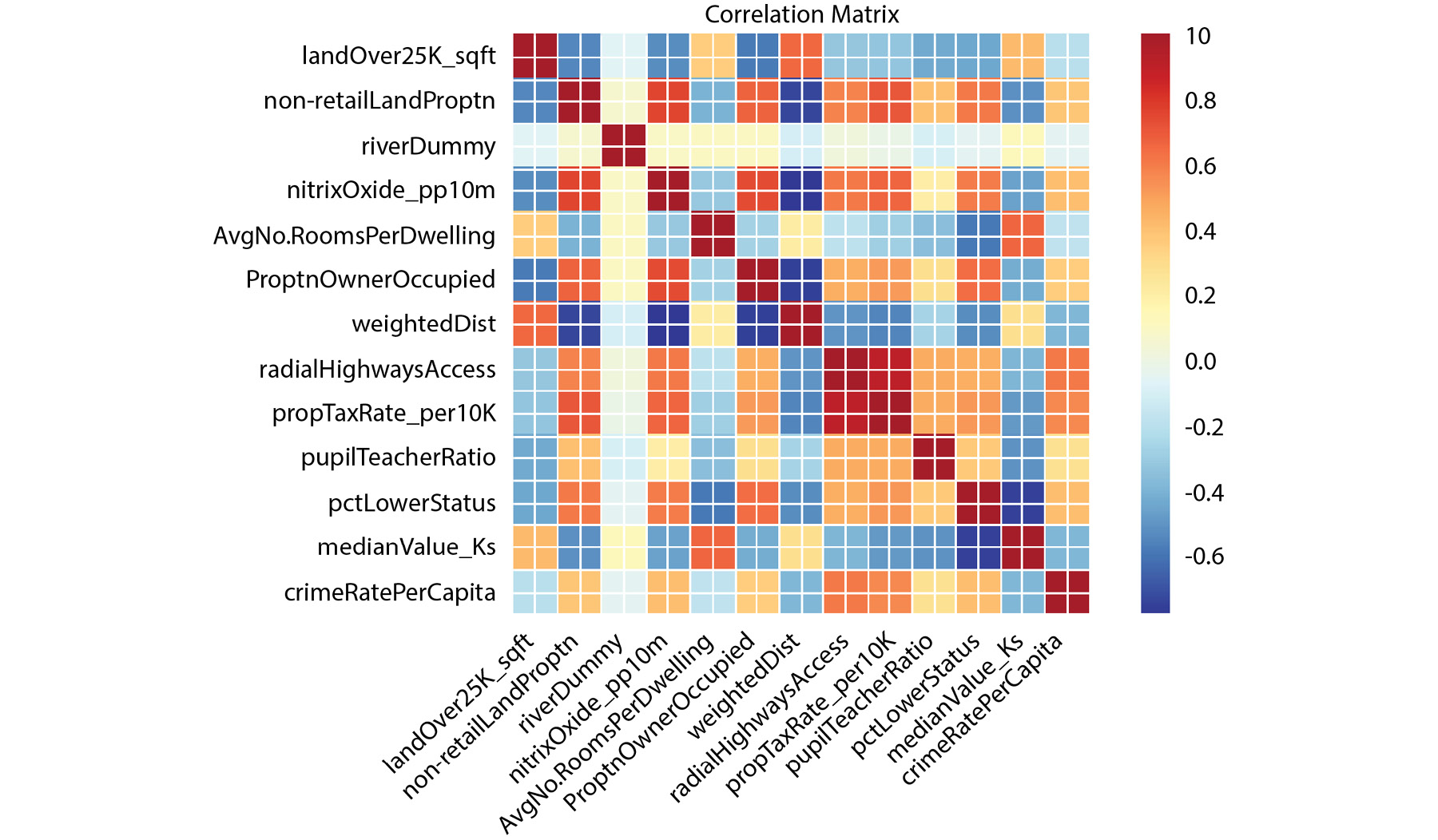
Figure 2.11: Output with the expected heatmap
In the preceding heatmap, we can see that there is a strong positive correlation (an increase in one causes an increase in the other) between variables that have orange or red squares. There is a strong negative correlation (an increase in one causes a decrease in the other) between variables with blue squares. There is little or no correlation between variables with pale-colored squares. For example, there appears to be a relatively strong correlation between nitrixOxide_pp10m and non-retailLandProptn, but a low correlation between riverDummy and any other variable.
We can use the findings from the correlation matrix as the starting point for further regression analysis. The heatmap gives us a good overview of relationships in the data and can show us which variables to target in our investigation.
The Correlation Coefficient
In the previous exercise, we have seen how a correlation matrix heatmap can be used to visualize the relationships between pairs of variables. We can also see these same relationships in numerical form using the raw correlation coefficient numbers. These are values between -1 and 1, which represent how closely two variables are linked.
Pandas provides a corr function, which when called on DataFrame provides a matrix (table) of the correlation of all numeric data types. In our case, running the code, train_data.corr (method = 'pearson'), in the Colab notebook provides the results in Figure 2.12.
It is important to note that Figure 2.12 is symmetric along the left diagonal. The left diagonal values are correlation coefficients for features against themselves (and so all of them have a value of one (1)), and therefore are not relevant to our analysis. The data in Figure 2.12 is what is presented as a plot in the output of Step 12 in Exercise 2.01.
You should get the following output:
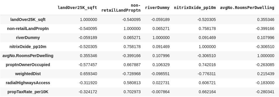
Figure 2.12: A correlation matrix of the training dataset
Note
The preceding output is truncated.
Data scientists use the correlation coefficient as a statistic in order to measure the linear relationship between two numeric variables, X and Y. The correlation coefficient for a sample of bivariate data is commonly represented by r. In statistics, the common method to measure the correlation between two numeric variables is by using the Pearson correlation coefficient. Going forward in this chapter, therefore, any reference to the correlation coefficient means the Pearson correlation coefficient.
To practically calculate the correlation coefficient statistic for the variables in our dataset in this course, we use a Python function. What is important to this discussion is the meaning of the values the correlation coefficient we calculate takes. The correlation coefficient (r) takes values between +1 and -1.
When r is equal to +1, the relationship between X and Y is such that both X and Y increase or decrease in the same direction perfectly. When r is equal to -1, the relationship between X and Y is such that an increase in X is associated with a decrease in Y perfectly and vice versa. When r is equal to zero (0), there is no linear relationship between X and Y.
Having no linear relationship between X and Y does not mean that X and Y are not related; instead, it means that if there is any relationship, it cannot be described by a straight line. In practice, correlation coefficient values around 0.6 or higher (or -0.6 or lower) is a sign of a potentially exciting linear relationship between two variables, X and Y.
The last column of the output of Exercise 2.01, Step 12, provides r values for crime rate per capita against other features in color shades. Using the color bar, it is obvious that radialHighwaysAccess, propTaxRate_per10K, nitrixOxide_pp10m, and pctLowerStatus have the strongest correlation with crime rate per capita. This indicates that a possible linear relationship, between crime rate per capita and any of these independent variables, may be worth looking into.
Exercise 2.02: Graphical Investigation of Linear Relationships Using Python
Scatter graphs fitted with a regression line are a quick way by which a data scientist can visualize a possible correlation between a dependent variable and an independent variable.
The goal of the exercise is to use this technique to investigate any linear relationship that may exist between crime rate per capita and the median value of owner-occupied homes in towns in the city of Boston.
The following steps will help you complete the exercise:
- Open a new Colab notebook file and execute the steps up to and including Step 11 from Exercise 2.01.
- Use the
subplotsfunction inmatplotlibto define a canvas (assigned the variable namefigin the following code) and a graph object (assigned the variable nameaxin the following code) in Python. You can set the size of the graph by setting thefigsize(width =10, height =6) argument of the function:fig, ax = plt.subplots(figsize=(10, 6))
- Use the
seabornfunctionregplotto create the scatter plot:sns.regplot(x='medianValue_Ks', y='crimeRatePerCapita', ci=None, data=train_data, ax=ax, color='k', scatter_kws={"s": 20,"color":\ "royalblue", "alpha":1})Note
The backslash(
\) in the following code is to tell Python that the line of code continues on the next line.The function accepts arguments for the independent variable (
x), the dependent variable (y), the confidence interval of the regression parameters (ci), which takes values from 0 to 100, the DataFrame that hasxandy(data), a matplotlib graph object (ax), and others to control the aesthetics of the points on the graph. (In this case, the confidence interval is set toNone– we will see more on confidence intervals later in the chapter.) - Set the
xandylabels, thefontsizeandnamelabels, thexandylimits, and thetickparameters of the matplotlib graph object (ax). Also, set the layout of the canvas totight:ax.set_ylabel('Crime rate per Capita', fontsize=15, fontname='DejaVu Sans') ax.set_xlabel("Median value of owner-occupied homes in $1000's",\ fontsize=15, fontname='DejaVu Sans') ax.set_xlim(left=None, right=None) ax.set_ylim(bottom=None, top=30) ax.tick_params(axis='both', which='major', labelsize=12) fig.tight_layout()You should get the following output:
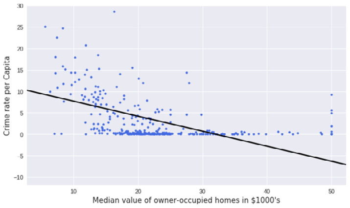
Figure 2.13: Scatter graph with a regression line using Python
If the exercise was followed correctly, the output must be the same as the graph in Figure 2.3. In Figure 2.3, this output was presented and used to introduce linear regression without showing how it was created. What this exercise has taught us is how to create a scatter graph and fit a regression line through it using Python.
Exercise 2.03: Examining a Possible Log-Linear Relationship Using Python
In this exercise, we will use the logarithm function to transform variables and investigate whether this helps provide a better fit of the regression line to the data. We will also look at how to use confidence intervals by including a 95% confidence interval of the regression coefficients on the plot.
The following steps will help you to complete this exercise:
- Open a new Colab notebook file and execute all the steps up to Step 11 from Exercise 2.01.
- Use the
subplotsfunction inmatplotlibto define a canvas and a graph object in Python:fig, ax = plt.subplots(figsize=(10, 6))
- Use the logarithm function in
numpy(np.log) to transform the dependent variable (y). This essentially creates a new variable,log(y):y = np.log(train_data['crimeRatePerCapita'])
- Use the seaborn
regplotfunction to create the scatter plot. Set theregplotfunction confidence interval argument (ci) to95%. This will calculate a95%confidence interval for the regression coefficients and have them plotted on the graph as a shaded area along the regression line. A confidence interval gives an estimated range that is likely to contain the true value that you're looking for. So, a95%confidence interval indicates we can be95%certain that the true regression coefficients lie in that shaded area. - Parse the
yargument with the new variable we defined in the preceding step. Thexargument is the original variable from the DataFrame without any transformation:sns.regplot(x='medianValue_Ks', y=y, ci=95, data=train_data, ax=ax, color='k', scatter_kws={"s": 20,"color": "royalblue", "alpha":1}) - Set the
xandylabels, thefontsizeandnamelabels, thexandylimits, and thetickparameters of thematplotlibgraph object (ax). Also, set the layout of the canvas totight:ax.set_ylabel('log of Crime rate per Capita', fontsize=15,\ fontname='DejaVu Sans') ax.set_xlabel("Median value of owner-occupied homes in $1000's",\ fontsize=15, fontname='DejaVu Sans') ax.set_xlim(left=None, right=None) ax.set_ylim(bottom=None, top=None) ax.tick_params(axis='both', which='major', labelsize=12) fig.tight_layout()The output is as follows:
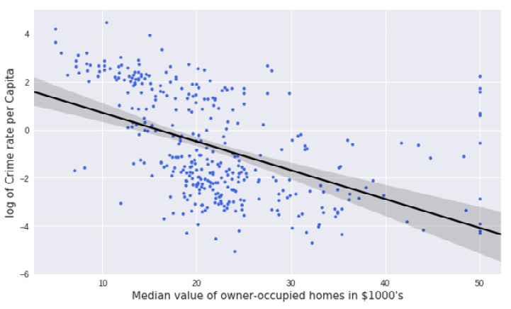
Figure 2.14: Expected scatter plot with an improved linear regression line
By completing this exercise, we have successfully improved our scatter plot. The regression line created in this activity fits the data better than what was created in Exercise 2.02. You can see by comparing the two graphs, the regression line in the log graph more clearly matches the spread of the data points. We have solved the issue where the bottom third of the line had no points clustered around it. This was achieved by transforming the dependent variable with the logarithm function. The transformed dependent variable (log of crime rate per capita) has an improved linear relationship with the median value of owner-occupied homes than the untransformed variable.
The Statsmodels formula API
In Figure 2.3, a solid line represents the relationship between the crime rate per capita and the median value of owner-occupied homes. But how can we obtain the equation that describes this line? In other words, how can we find the intercept and the slope of the straight-line relationship?
Python provides a rich Application Programming Interface (API) for doing this easily. The statsmodels formula API enables the data scientist to use the formula language to define regression models that can be found in statistics literature and many dedicated statistical computer packages.
Exercise 2.04: Fitting a Simple Linear Regression Model Using the Statsmodels formula API
In this exercise, we examine a simple linear regression model where the crime rate per capita is the dependent variable and the median value of owner-occupied homes is the independent variable. We use the statsmodels formula API to create a linear regression model for Python to analyze.
The following steps will help you complete this exercise:
- Open a new Colab notebook file and import the required packages.
import pandas as pd
import statsmodels.formula.api as smf
from sklearn.model_selection import train_test_split
- Execute Step 2 to 11 from Exercise 2.01.
- Define a linear regression model and assign it to a variable named
linearModel:linearModel = smf.ols(formula='crimeRatePerCapita ~ medianValue_Ks',\ data=train_data)
As you can see, we call the
olsfunction of the statsmodels API and set its formula argument by defining apatsyformula string that uses the tilde (~) symbol to relate the dependent variable to the independent variable. Tell the function where to find the variables named, in the string, by assigning the data argument of theolsfunction to the DataFrame that contains your variables (train_data). - Call the .
fitmethod of the model instance and assign the results of the method to alinearModelResultvariable, as shown in the following code snippet:linearModelResult = linearModel.fit()
- Print a summary of the results stored the
linearModelResultvariable by running the following code:print(linearModelResult.summary())
You should get the following output:
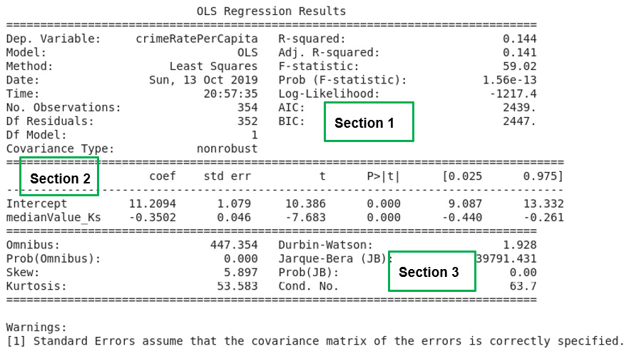
Figure 2.15: A summary of the simple linear regression analysis results
If the exercise was correctly followed, then a model has been created with the statsmodels formula API. The fit method (.fit()) of the model object was called to fit the linear regression model to the data. What fitting here means is to estimate the regression coefficients (parameters) using the ordinary least squares method.
Analyzing the Model Summary
The .fit method provides many functions to explore its output. These include the conf_int(), pvalues, tvalues, and summary() parameters. With these functions, the parameters of the model, the confidence intervals, and the p-values and t-values for the analysis can be retrieved from the results. (The concept of p-values and t-values will be explained later in the chapter.)
The syntax simply involves following the dot notation, after the variable name containing the results, with the relevant function name – for example, linearModelResult.conf_int() will output the confidence interval values. The handiest of them all is the summary() function, which presents a table of all relevant results from the analysis.
In Figure 2.15, the output of the summary function used in Exercise 2.04 is presented. The output of the summary function is divided, using double dashed lines, into three main sections.
In Chapter 9, Interpreting a Machine Learning Model, the results of the three sections will be treated in detail. However, it is important to comment on a few points here.
In the top-left corner of Section 1 in Figure 2.15, we find the dependent variable in the model (Dep. Variable) printed and crimeRatePerCapita is the value for Exercise 2.04. A statistic named R-squared with a value of 0.144 for our model is also provided in Section 1. The R-squared value is calculated by Python as a fraction (0.144) but it is to be reported in percentages so the value for our model is 14.4% The R-squared statistic provides a measure of how much of the variability in the dependent variable (crimeRatePerCapita), our model is able to explain. It can be interpreted as a measure of how well our model fits the dataset. In Section 2 of Figure 2.15, the intercept and the independent variable in our model is reported. The independent variable in our model is the median value of owner-occupied homes (medianValue_Ks).
In this same Section 2, just next to the intercept and the independent variable, is a column that reports the model coefficients (coef). The intercept and the coefficient of the independent variable are printed under the column labeled coef in the summary report that Python prints out. The intercept has a value of 11.2094 with the coefficient of the independent variable having a value of negative 0.3502 (-0.3502). If we choose to denote the dependent variable in our model (crimeRatePerCapita) as y and the independent variable (the median value of owner-occupied homes) as x, we have all the ingredients to write out the equation that defines our model.
Thus, y ≈ 11.2094 - 0.3502 x, is the equation for our model. In Chapter 9, Interpreting a Machine Learning Model, what this model means and how it can be used will be discussed in full.
The Model Formula Language
Python is a very powerful language liked by many developers. Since the release of version 0.5.0 of statsmodels, Python now provides a very competitive option for statistical analysis and modeling rivaling R and SAS.
This includes what is commonly referred to as the R-style formula language, by which statistical models can be easily defined. Statsmodels implements the R-style formula language by using the Patsy Python library internally to convert formulas and data to the matrices that are used in model fitting.
Figure 2.16 summarizes the operators used to construct the Patsy formula strings and what they mean:
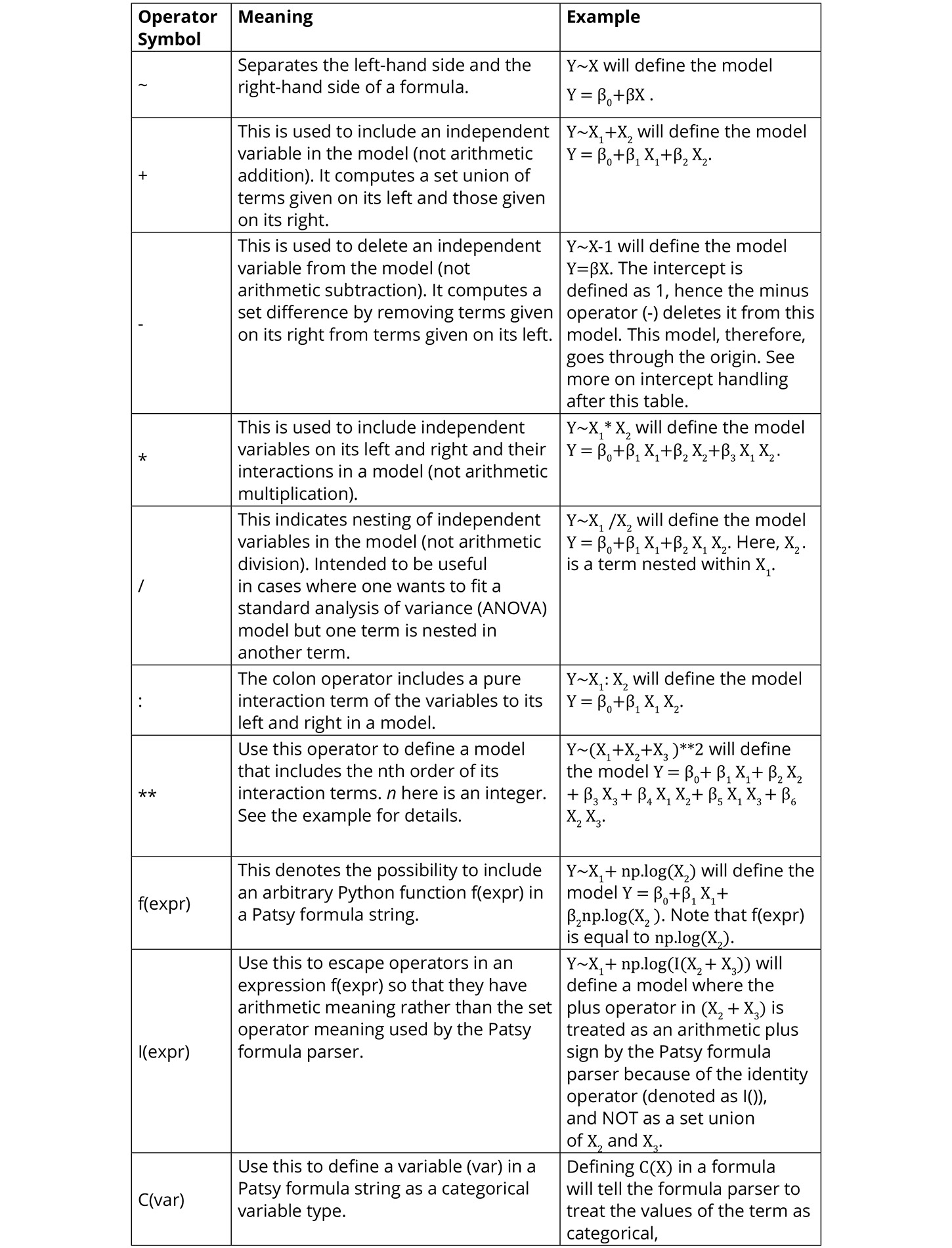
Figure 2.16: A summary of the Patsy formula syntax and examples
Intercept Handling
In patsy formula strings, string 1 is used to define the intercept of a model. Because the intercept is needed most of the time, string 1 is automatically included in every formula string definition. You don't have to include it in your string to specify the intercept. It is there invisibly. If you want to delete the intercept from your model, however, then you can subtract one (-1) from the formula string and that will define a model that passes through the origin. For compatibility with other statistical software, Patsy also allows the use of the string zero (0) and negative one (-1) to be used to exclude the intercept from a model. What this means is that, if you include 0 or -1 on the right-hand side of your formula string, your model will have no intercept.
Activity 2.01: Fitting a Log-Linear Model Using the Statsmodels formula API
You have seen how to use the statsmodels API to fit a linear regression model. In this activity, you are asked to fit a log-linear model. Your model should represent the relationship between the log-transformed dependent variable (log of crime rate per capita) and the median value of owner-occupied homes.
The steps to complete this activity are as follows:
- Define a linear regression model and assign it to a variable. Remember to use the
logfunction to transform the dependent variable in the formula string. - Call the
fitmethod of the model instance and assign the results of the method to a variable. - Print a summary of the results and analyze the output.
Your output should look like the following figure:
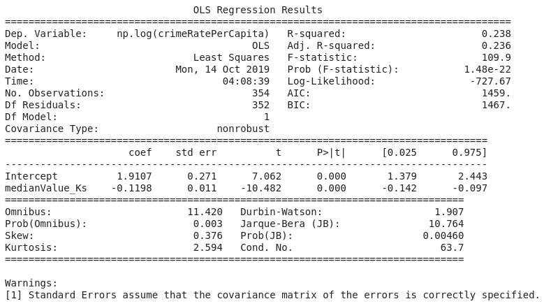
Figure 2.17: A log-linear regression of crime rate per capita on the median value of owner-occupied homes
Note
The solution to this activity can be found here: https://packt.live/2GbJloz.


