Exploring GoogLeNet and Inception v3
As we have discovered the progression of CNN models from LeNet to VGG so far, we have observed the sequential stacking of more convolutional and fully connected layers. This resulted in deep networks with a lot of parameters to train. GoogLeNet emerged as a radically different type of CNN architecture that is composed of a module of parallel convolutional layers called the inception module. Because of this, GoogLeNet is also called Inception v1 (v1 marked the first version as more versions came along later). Some of the drastically new elements introduced by GoogLeNet were the following:
- The inception module – a module of several parallel convolutional layers
- Using 1x1 convolutions to reduce the number of model parameters
- Global average pooling instead of a fully connected layer – reduces overfitting
- Using auxiliary classifiers for training – for regularization and gradient stability
GoogLeNet has 22 layers, which is more than the number of layers of any VGG model variant. Yet, due to some of the optimization tricks used, the number of parameters in GoogLeNet is 5 million, which is far less than the 138 million parameters of VGG. Let’s expand on some of the key features of this model.
Inception modules
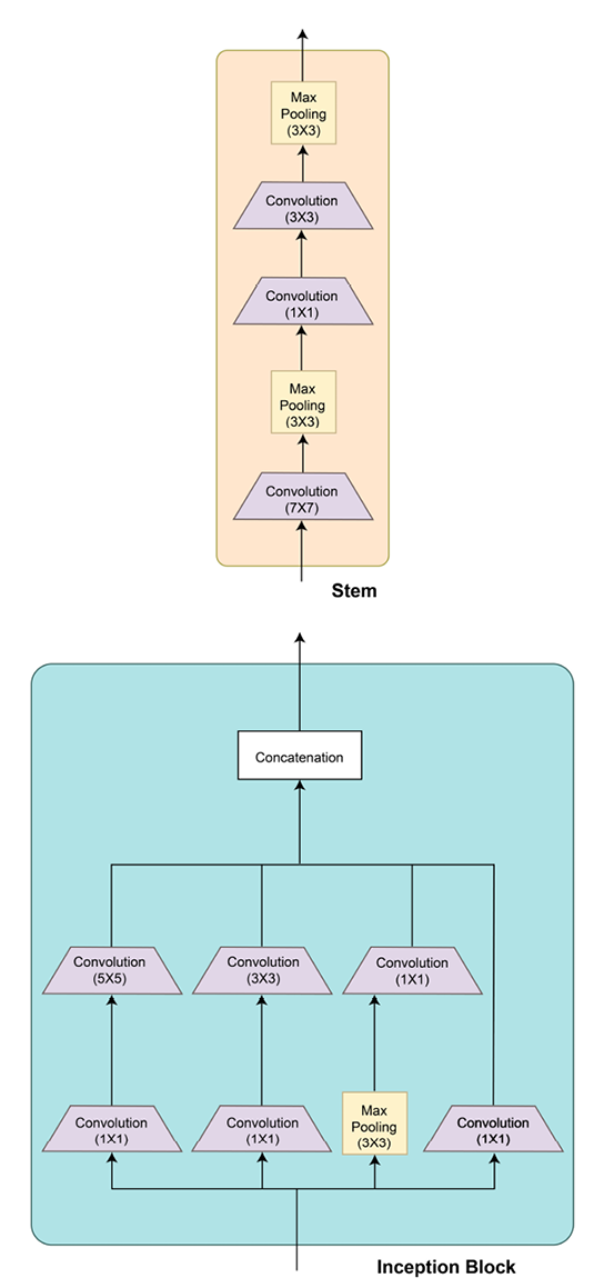
Perhaps the single most important contribution of this model was the development of a convolutional module with several convolutional layers running in parallel, which are finally concatenated to produce a single output vector. These parallel convolutional layers operate with different kernel sizes ranging from 1x1 to 3x3 to 5x5. The idea is to extract all levels of visual information from the image. Besides these convolutions, a 3x3 max pooling layer adds another level of feature extraction.
Figure 2.14 shows the inception block diagram along with the overall GoogLeNet architecture:


Figure 2.14: GoogLeNet architecture
By using this architecture diagram, we can build the inception module in PyTorch as shown here:
class InceptionModule(nn.Module):
    def __init__(self, input_planes, n_channels1x1, n_channels3x3red,
                 n_channels3x3, n_channels5x5red, n_channels5x5,
                 pooling_planes):
        super(InceptionModule, self).__init__()
        # 1x1 convolution branch
        self.block1 = nn.Sequential(
            nn.Conv2d(input_planes, n_channels1x1, kernel_size=1),
                      nn.BatchNorm2d(n_channels1x1),nn.ReLU(True),)
        # 1x1 convolution -> 3x3 convolution branch
        self.block2 = nn.Sequential(
            nn.Conv2d(input_planes, n_channels3x3red, kernel_size=1),
            nn.BatchNorm2d(n_channels3x3red),
            nn.ReLU(True), nn.Conv2d(n_channels3x3red, n_channels3x3,
                                     kernel_size=3, padding=1),
                                     nn.BatchNorm2d(n_channels3x3),
                                     nn.ReLU(True),)
        # 1x1 conv -> 5x5 conv branch
        self.block3 = nn.Sequential(
            nn.Conv2d(input_planes, n_channels5x5red, kernel_size=1),
            nn.BatchNorm2d(n_channels5x5red),
            nn.ReLU(True), nn.Conv2d(n_channels5x5red, n_channels5x5,
                                     kernel_size=3, padding=1),
                                     nn.BatchNorm2d(n_channels5x5),
                                     nn.ReLU(True),
            nn.Conv2d(n_channels5x5, n_channels5x5,
                      kernel_size=3, padding=1),
                      nn.BatchNorm2d(n_channels5x5),
                      nn.ReLU(True),)
        # 3x3 pool -> 1x1 conv branch
        self.block4 = nn.Sequential(
            nn.MaxPool2d(3, stride=1, padding=1),
            nn.Conv2d(input_planes, pooling_planes, kernel_size=1),
            nn.BatchNorm2d(pooling_planes),
            nn.ReLU(True),)
    def forward(self, ip):
        op1 = self.block1(ip)
        op2 = self.block2(ip)
        op3 = self.block3(ip)
        op4 = self.block4(ip)
        return torch.cat([op1,op2,op3,op4], 1)
Next, we will look at another important feature of GoogLeNet – 1x1 convolutions.
1x1 convolutions
In addition to the parallel convolutional layers in an inception module, each parallel layer has a preceding 1x1 convolutional layer. The reason behind using these 1x1 convolutional layers is dimensionality reduction. 1x1 convolutions do not change the width and height of the image representation but can alter the depth of an image representation. This trick is used to reduce the depth of the input visual features before performing the 1x1, 3x3, and 5x5 convolutions parallelly. Reducing the number of parameters not only helps build a lighter model but also combats overfitting.
Global average pooling
If we look at the overall GoogLeNet architecture in Figure 2.14, the penultimate output layer of the model is preceded by a 7x7 average pooling layer. This layer again helps in reducing the number of parameters of the model, thereby reducing overfitting. Without this layer, the model would have millions of additional parameters due to the dense connections of a fully connected layer.
Auxiliary classifiers
Figure 2.14 also shows two extra or auxiliary output branches in the model. These auxiliary classifiers are supposed to tackle the vanishing gradient problem by adding to the gradients’ magnitude during backpropagation, especially for the layers toward the input end. Because these models have a large number of layers, vanishing gradients can become a major limitation. Hence, using auxiliary classifiers has proven useful for this 22-layer deep model. Additionally, the auxiliary branches also help in regularization. Please note that these auxiliary branches are switched off/discarded while making predictions.
Once we have the inception module defined using PyTorch, we can easily instantiate the entire Inception v1 model as follows:
class GoogLeNet(nn.Module):
    def __init__(self):
        super(GoogLeNet, self).__init__()
        self.stem = nn.Sequential(
            nn.Conv2d(3, 192, kernel_size=3, padding=1),
            nn.BatchNorm2d(192),
            nn.ReLU(True),)
        self.im1 = InceptionModule(192,  64,  96, 128, 16, 32, 32)
        self.im2 = InceptionModule(256, 128, 128, 192, 32, 96, 64)
        self.max_pool = nn.MaxPool2d(3, stride=2, padding=1)
        self.im3 = InceptionModule(480, 192,  96, 208, 16,  48,  64)
        self.im4 = InceptionModule(512, 160, 112, 224, 24,  64,  64)
        self.im5 = InceptionModule(512, 128, 128, 256, 24,  64,  64)
        self.im6 = InceptionModule(512, 112, 144, 288, 32,  64,  64)
        self.im7 = InceptionModule(528, 256, 160, 320, 32, 128, 128)
        self.im8 = InceptionModule(832, 256, 160, 320, 32, 128, 128)
        self.im9 = InceptionModule(832, 384, 192, 384, 48, 128, 128)
        self.average_pool = nn.AvgPool2d(7, stride=1)
        self.fc = nn.Linear(4096, 1000)
    def forward(self, ip):
        op = self.stem(ip)
        out = self.im1(op)
        out = self.im2(op)
        op = self.maxpool(op)
        op = self.a4(op)
        op = self.b4(op)
        op = self.c4(op)
        op = self.d4(op)
        op = self.e4(op)
        op = self.max_pool(op)
        op = self.a5(op)
        op = self.b5(op)
        op = self.avgerage_pool(op)
        op = op.view(op.size(0), -1)
        op = self.fc(op)
        return op
Besides instantiating our own model, we can always load a pretrained GoogLeNet with just two lines of code:
import torchvision.models as models
model = models.googlenet(pretrained=True)
Finally, as mentioned earlier, a number of versions of the Inception model were developed later. One of the eminent ones was Inception v3, which we will briefly discuss next.
Inception v3
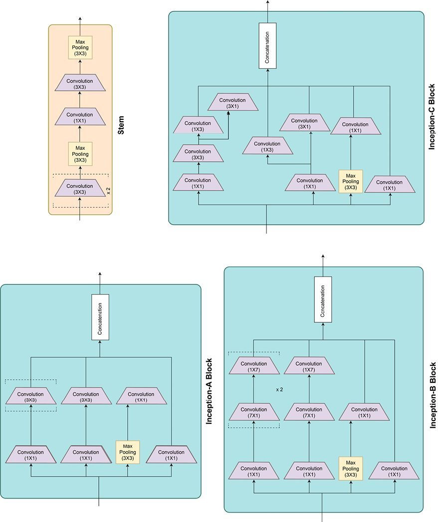
This successor of Inception v1 has a total of 24 million parameters as compared to 5 million in v1. Besides the addition of several more layers, this model introduced different kinds of inception modules, which are stacked sequentially.
Figure 2.15 shows the different inception modules and the full model architecture:


Figure 2.15: Inception v3 architecture
It can be seen from the architecture that this model is an architectural extension of the Inception v1 model. Once again, besides building the model manually, we can use the pretrained model from PyTorch’s repository as follows:
import torchvision.models as models
model = models.inception_v3(pretrained=True)
In the next section, we will go through the classes of CNN models that have effectively combatted the vanishing gradient problem in very deep CNNs – ResNet and DenseNet. We will learn about the novel techniques of skip connections and dense connections and use PyTorch to code the fundamental modules behind these advanced architectures.


