Search icon CANCEL
Subscription
0
Cart icon
Your Cart (0 item)
Close icon
You have no products in your basket yet
Save more on your purchases! discount-offer-chevron-icon
Savings automatically calculated. No voucher code required.
Arrow left icon
Explore Products
Best Sellers
New Releases
Books
Videos
Audiobooks
Learning Hub
Free Learning
Arrow right icon
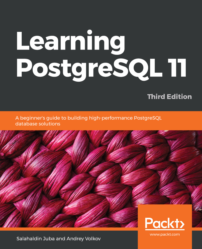
Learning PostgreSQL 11

Learning PostgreSQL 11: A beginner's guide to building high-performance PostgreSQL database solutions , Third Edition

Arrow left icon
Profile Icon Christopher Travers Profile Icon Volkov
Arrow right icon
€32.99
Full star icon Full star icon Half star icon Empty star icon Empty star icon 2.7 (6 Ratings)
Paperback Jan 2019 556 pages 3rd Edition
eBook
€8.99 €26.99
Paperback
€32.99
Subscription
Free Trial
Renews at €18.99p/m
eBook
€8.99 €26.99
Paperback
€32.99
Subscription
Free Trial
Renews at €18.99p/m

What do you get with Print?

Product feature icon Instant access to your digital eBook copy whilst your Print order is Shipped
Product feature icon Paperback book shipped to your preferred address
Product feature icon Download this book in EPUB and PDF formats
Product feature icon Access this title in our online reader with advanced features
Product feature icon DRM FREE - Read whenever, wherever and however you want
Product feature icon AI Assistant (beta) to help accelerate your learning
OR
Modal Close icon
Payment Processing...
tick Completed

Shipping Address

Billing Address

Shipping Methods
Table of content icon View table of contents Preview book icon Preview Book

Learning PostgreSQL 11

Relational Databases

This chapter, and the ones following, will provide a high-level overview of topics related to database development. These topics will cover the theoretical aspects of relational databases. The first two chapters try to summarize theoretical topics that are seen on a daily basis. Understanding these theoretical concepts will enable developers to not only come up with clean designs but also to master relational databases.

This chapter is not restricted to learning PostgreSQL, but covers all relational databases. The topics covered in this chapter include the following:

  • Database management systems
  • Relational algebra
  • Data modeling

Database management systems

Different database management systems (DBMS) support diverse application scenarios, use cases, and requirements. DBMS have a long history. First, we will quickly take a look at the recent history, and then explore the market-dominant database management system categories.

A brief history

Broadly, the term database can be used to present a collection of things. Moreover, this term brings to mind many other terms including data, information, data structure, and management. A database can be defined as a collection or repository of data, which has a certain structure, managed by a DBMS. Data can be structured as tabular data, semi-structured as XML documents, or unstructured data that does not fit a predefined data model.

In the early days, databases were mainly aimed at supporting business applications; this led us to the well-defined relational algebra and relational database systems. With the introduction of object-oriented languages, new paradigms of DBMS appeared, such as object-relational databases and object-oriented databases. Also, many businesses, as well as scientific applications, use arrays, images, and spatial data; thus, new models such as raster, map, and array algebra are supported. Graph databases are used to support graph queries such as the shortest path from one node to another, along with supporting traversal queries easily.

With the advent of web applications such as social portals, it is now necessary to support a huge number of requests in a distributed manner. This has led to another new paradigm of databases called Not Only SQL (NoSQL), which has different requirements, such as performance over fault tolerance and horizontal scaling capabilities. In general, the timeline of database evolution was greatly affected by many factors, such as the following:

  • Functional requirements: The nature of the applications using a DBMS led to the development of extensions on top of relational databases such as PostGIS (for spatial data), or even a dedicated DBMS such as SciDB (for scientific data analytics).
  • Nonfunctional requirements: The success of object-oriented programming languages has created new trends such as object-oriented databases. Object-relational DBMS have appeared to bridge the gap between relational databases and the object-oriented programming languages. Data explosion and the necessity to handle terabytes of data on commodity hardware have led to database systems that can easily scale up horizontally.

Database categories

Many database models have appeared and vanished, such as the network model and the hierarchical model. The predominant categories now in the market are relational, object-relational, and NoSQL databases. One should not think of NoSQL and SQL databases as rivals; they are complementary to each other. By utilizing different database systems, one can overcome many limitations and get the best of different technologies.

NoSQL databases can provide great benefits such as availability, schema-free, and horizontal scaling, but they also have limitations such as performance, data retrieval constraints, and learning time. Relational databases often adhere to SQL as defined by ISO. SQL is a very expressive and extremely powerful tool for retrieving data in different forms. Many NoSQL databases such as Cassandra lack the capability to retrieve data as in relational databases.

NoSQL databases

NoSQL databases are affected by the CAP theorem, also known as Brewer's theorem. In 2002, S. Gilbert and N. Lynch published a formal proof of the CAP theorem in their article Brewer's conjecture and the feasibility of consistent, available, partition-tolerant web services. In 2009, the NoSQL movement began. Currently, there are over 150 NoSQL databases (nosql-database.org).

The CAP theorem

The CAP theorem states that it is impossible for a distributed computing system to simultaneously provide all three of the following guarantees:

  • Consistent: All clients see (immediately) the latest data even in the case of updates.
  • Available: All clients can find a replica of some data even in the case of a node failure. This means that even if some part of the system goes down, the clients can still access consistent and valid data.
  • Partition tolerance: The system continues to work regardless of arbitrary message loss or failure of part of the system.

The choice of which features to discard determines the nature of the system. For example, one could sacrifice consistency to get a scalable, simple, and high-performance database management system. Often, the main difference between a relational database and a NoSQL database is consistency. A relational database enforces atomicity, consistency, isolation, and durability (ACID) properties. In contrast, many NoSQL databases adopt the basically available, soft-state, eventual consistency (BASE) model.

NoSQL motivation

A NoSQL database does not entity relation model for data storage, manipulation, and retrieval. NoSQL databases are often distributed, open source, and horizontally scalable. NoSQL often adopts the base model, which prizes availability over consistency, and informally guarantees that if no new updates are made on a data item, eventually all access to that data item will return the latest version of that data item. The advantages of this approach include the following:

  • Simplicity of design
  • Horizontal scaling and easy replication
  • Schema-free
  • A huge amount of data support

We will now explore a few types of NoSQL databases.

Key-value databases

The key-value store is the simplest database store. In this database model, the storage, as its name suggests, is based on maps or hash tables. Some key-value databases allow complex values to be stored as lists and hash tables. Key-value pairs are extremely fast for certain scenarios but lack the support for complex queries and aggregation. Some of the existing open source key-value databases are Riak, Redis, Couchbase Server, and MemcacheDB.

Columnar databases

Columnar or column-oriented databases are based on columns. Data in a certain column in a two-dimensional relation is stored together.

Unlike relational databases, adding columns is inexpensive and is done on a row-by-row basis. Rows can have a different set of columns. Tables can benefit from this structure by eliminating the storage cost of the null values. This model is best suited for distributed databases.

HBase is one of the most famous columnar databases. It is based on the Google Bigtable storage system. Column-oriented databases are designed for huge data scenarios, so they scale up easily. For example, Facebook uses HBase to power their message infrastructure. For small datasets, HBase is not a suitable architecture. First, the recommended hardware topology for HBase is a five-node server deployment. Also, it needs a lot of administration and is difficult to learn and master.

Document databases

A document-oriented database is suitable for documents and semi-structured data. The central concept of a document-oriented database is the notion of a document. Documents encapsulate and encode data (or information) in some standard formats or encodings such as XML, JSON, and BSON. Documents do not adhere to a standard schema or have the same structure, so they provide a high degree of flexibility. Unlike relational databases, changing the structure of the document is simple and does not lock the clients from accessing the data.

Document databases merge the power of relational databases and column-oriented databases. They provide support for ad hoc queries and can be scaled up easily. Depending on the design of the document database, MongoDB is designed to handle a huge amount of data efficiently. On the other hand, CouchDB provides high availability even in the case of hardware failure.

Graph databases

Graph databases are based on graph theory, where a database consists of nodes and edges. The nodes, as well as the edges, can be assigned data. Graph databases allow traversing between the nodes using edges. As a graph is a generic data structure, graph databases are capable of representing different data. A famous implementation of an open source, commercially supported graph database is Neo4j.

Relational and object-relational databases

Relational DBMS are one of the most widely used DBMSes in the world. It is highly unlikely that any organization, institution, or personal computer today does not have or use a piece of software that relies on RDBMS.

Software applications can use relational databases via dedicated database servers or via lightweight RDBMS engines, embedded in the software applications as shared libraries.

The capabilities of a relational database management system vary from one vendor to another, but most of them adhere to the American National Standards Institute (ANSI) SQL standards. A relational database is formally described by relational algebra, and is based on the relational model. Object-relational databases (ORDs) are similar to relational databases. They support the following object-oriented model concepts:

  • User-defined and complex data types
  • Inheritance

ACID properties

In a relational database, a single logical operation is called a transaction. The technical translation of a transaction is a set of database operations, which are create, read, update, and delete (CRUD). An example of explaining a transaction is a budget assignment to several projects in the company assuming we have a fixed amount of money. If we increase a certain project budget, we need to deduct this amount of increase from another project. The ACID properties in this context could be described as follows:

  • Atomicity: All or nothing, which means that if a part of a transaction fails, then the transaction fails as a whole.
  • Consistency: Any transaction gets the database from one valid state to another valid state. Database consistency is governed normally by data constraints and the relation between data and any combination thereof. For example, imagine if someone would like to completely purge his account on a shopping service. In order to purge his account, his account details, such as a list of addresses, will also need to be purged. This is governed by foreign key constraints, which will be explained in detail in the coming chapter.
  • Isolation: Concurrent execution of transactions results in a system state that would be obtained if the transactions were executed serially.
  • Durability: The transactions that are committed—that is, executed successfully—are persistent even with power loss or some server crashes. In PostgreSQL, this is done normally by a technique called Write-Ahead Logging (WAL). Another database refers to this as a transaction log such as in Oracle.

The SQL language

Relational databases are often linked to Structured Query Language (SQL). SQL is a declarative programming language and is the standard relational database language. The ANSI and the International Organization for Standardization (ISO) published the SQL standard for the first time in 1986, followed by many versions such as SQL:1999, SQL:2003, SQL:2006, SQL:2008, SQL:2011, and SQL:2016.

The SQL language has several parts:

  • Data definition language (DDL): It defines and amends the relational structure
  • Data manipulation language (DML): It retrieves and extracts information from the relations
  • Data control language (DCL): It controls the access rights to relations

Relational model concepts

A relational model is a first-order predicate logic that was first introduced by Edgar F. Codd in 1970 in his paper A Relational Model of Data for Large Shared Data Banks. A database is represented as a collection of relations. The state of the whole database is defined by the state of all the relations in the database. Different information can be extracted from the relations by joining and aggregating data from different relations and by applying filters on the data. In this section, the basic concepts of the relational model are introduced using the top-down approach by first describing the relation, tuple, attribute, and domain.

The terms relation, tuple, attribute, and unknown, which are used in the formal relational model, are equivalent to table, row, column, and null in the SQL language.

Relation

Think of a relation as a table with a header, columns, and rows. The table name and the header help in interpreting the data in the rows. Each row represents a group of related data, which points to a certain object.

A relation is represented by a set of tuples. Tuples should have the same set of ordered attributes. Attributes have a domain, that is, a type and a name:

customer_id

first_name

last_name

email

Tuple →

1

thomas

sieh

thomas@example.com

Tuple →

2

wang

kim

kim@example.com

Attribute ↑

Attribute ↑

Attribute ↑

Attribute ↑

The relation schema is denoted by the relation name and the relation attributes. For example, customer (customer_id, first_name, last_name, and email) is the relation schema for the customer relation. Relation state is defined by the set of relation tuples; thus, adding, deleting, and amending a tuple will change the relation to another state.

Tuple order or position in the relation is not important, and the relation is not sensitive to tuple order. The tuples in the relation could be ordered by a single attribute or a set of attributes. Also, a relation cannot have duplicate tuples.

A relation can represent entities in the real world, such as a customer, or can be used to represent an association between relations. For example, the customer could have several services and a service can be offered to several customers. This could be modeled by three relations: customer, service, and customer_service. The customer_service relation associates the customer and the service relations. Separating the data in different relations is a key concept in relational database modeling, and is called normalization. Normalization is the process of organizing relation columns and relations to reduce data redundancy. For example, assume that a collection of services is stored in the customer relation. If a service is assigned to multiple customers, this would result in data redundancy. Also, updating a certain service would require updating all its copies in the customer table.

Tuple

A tuple is a set of ordered attributes. They are written by listing the elements within parentheses () and separated by commas, such as (john, smith, 1971). Tuple elements are identified via the attribute name. Tuples have the following properties:

  • (a1,a2, a3,…,an) = (b1, b2,b3,…,bn ) if and only if a1= b1, a2=b2, …,an= bn
  • A tuple is not a set; the order of attributes matters as well as duplicate members:
    • (a1, a2) ≠(a2, a1)
    • (a1, a1) ≠(a1)
  • A tuple has a finite set of attributes

In the formal relational model, multi-valued attributes, as well as composite attributes, are not allowed. This is important to reduce data redundancy and increase data consistency. This isn't strictly true in modern relational database systems because of the utilization of complex data types such as JSON and key-value stores.

There is a lot of debate regarding the application of normalization; the rule of thumb is to apply normalization unless there is a good reason not to do so.

The null value

Predicates in relational databases use three-valued logic (3VL), where there are three truth values: true, false, and null,. In a relational database, the third value, null, can be interpreted in many ways, such as unknown data, missing data, not applicable, or will be loaded later. The 3VL is used to remove ambiguity. For example, no two null values are equal.

In the next chapter, you will learn how to connect to the database and run queries. Now, I would like to show how a logical OR/AND truth table can be generated by the SQL language:

Logical AND and OR operators are commutative, that is, A AND B = B AND A.
\pset null null
WITH data (v) as (VALUES (true), (false),(null))
SELECT DISTINCT
first.v::TEXT as a,
second.v::TEXT as b,
(first.v AND second.v)::TEXT AS "a and b",
(first.v OR second.v)::TEXT as "a or b"
FROM
data as first cross join
data as second
ORDER BY a DESC nulls last, b DESC nulls last;
a | b | a and b | a or b
-------+-------+---------+--------
true | true | true | true
true | false | false | true
true | null | null | true
false | true | false | true
false | false | false | false
false | null | false | null
null | true | null | true
null | false | false | null
null | null | null | null
(9 rows)

The following table, which is generated by SQL, shows the NOT truth operator:

WITH data (v) as (VALUES (true), (false),(null)) SELECT v::text as a, (NOT v)::text as "NOT a" FROM data order by a desc nulls last;
a | NOT a
-------+-------
true | false
false | true
null | null
(3 rows)

Attribute

Each attribute has a name and a domain, and the name should be distinct within the relation. The domain defines the possible set of values that the attribute can have. One way to define the domain is to define the data type and a constraint on this data type. For example, the hourly wage should be a positive real number and bigger than five if we assume that the minimum hourly wage is five dollars. The domain could be continuous, such as salary, which is any positive real number, or discrete, such as gender.

The formal relational model puts a constraint on the domain: the value should be atomic. Atomicity means that each value in the domain is indivisible. For instance, the name attribute domain is not atomic because it can be divided into first name and last name. Some examples of domains are as follows:

  • Phone number: Numeric text with a certain length.
  • Country code: Defined by ISO 3166 as a list of two-letter codes (ISO alpha-2) and three-letter codes (ISO alpha-3). The country codes for Germany are DE and DEU for alpha-2 and alpha-3 respectively.
In real-life applications, it is better to use ISO and international standards for lookup tables such as country and currency. This enables you to expose your data much more easy to third-party software and increases your data quality.

Constraint

The relational model defines many constraints in order to control data integrity, redundancy, and validity. Here are some examples of checking for data:

  • Redundancy: Duplicate tuples are not allowed in the relation.
  • Validity: Check constraints and domain constraints are used to validate the data input, for example, the date of birth should be a date that occurred in the past.
  • Integrity: The relations within a single database are linked to each other. An action on a relation such as updating or deleting a tuple might leave the other relations in an invalid state.

We could classify the constraints in a relational database roughly into two categories:

  • Inherited constraints from the relational model: Domain integrity, entity integrity, and referential integrity constraints.
  • Semantic constraint, business rules, and application-specific constraints: These constraints cannot be expressed explicitly by the relational model. However, with the introduction of procedural SQL languages such as PL/pgSQL for PostgreSQL, relational databases can also be used to model these constraints.

Domain integrity constraint

The domain integrity constraint ensures data validity. The first step in defining the domain integrity constraint is to determine the appropriate data type. The domain data types could be an integer, real, boolean, character, text, inet, and so on. For example, the data type of the first name and email address is text. After specifying the data type, check constraints, such as the mail address pattern, need to be defined:

  • Check constraint: A check constraint can be applied to a single attribute or a combination of many attributes in a tuple. Let's assume that the customer_service schema is defined as customer_id, service_id, start_date, end_date, and order_date. For this relation, we can have a check constraint to make sure that start_date and end_date are entered correctly by applying the following check: start_date is less than end_date.
  • Default constraint: The attribute can have a default value. The default value could be a fixed value such as the default hourly wage of the employees, for example, $10. It may also have a dynamic value based on a function such as random, current time, and date. For example, in the customer_service relation, order_date can have a default value, which is the current date.
  • Unique constraint: A unique constraint guarantees that the attribute has a distinct value in each tuple. It allows null values. For example, let's assume that we have a relation player defined as a player (player_id, player_nickname). The player uses his ID to play with others; he can also pick up a nickname, which is also unique to identify himself.
  • Not null constraint: By default, the attribute value can be null. The not null constraint prevents an attribute from having a null value. For example, each person in the birth registry record should have a name.

Entity integrity constraint

In the relational model, a relation is defined as a set of tuples. This means that all the tuples in a relation must be distinct. The entity integrity constraint is enforced by having a primary key, which is an attribute/set of attributes with the following characteristics:

  • The attribute should be unique
  • The attributes should be not null

Each relation must have only one primary key, but can have many unique keys. A candidate key is a minimal set of attributes that can identify a tuple. All unique, not null attributes can be candidate keys. The set of all attributes form a super key. In practice, we often pick up a single attribute to be a primary key instead of a compound key (a key that consists of two or more attributes that uniquely identify a tuple) to simplify the joining of the relations with each other.

If the primary key is generated by the DBMS, then it is called a surrogate key or synthetic key. Otherwise, it is called a natural key. The surrogate key candidates can be sequences and universal unique identifiers (UUIDs). A surrogate key has many advantages such as performance, requirement change tolerance, agility, and compatibility with object-relational mappers. The chief disadvantage of surrogate keys is that it makes redundant tuples possible.

A sequence is a number generator that is used to generate a series of numbers based on the current number's value. This term is used mainly in PostgreSQL and Oracle databases. PostgreSQL also has an identity column, which is mainly used to generate series of numbers. More about this topic is explained in Chapter 4, PostgreSQL Advanced Building Blocks.

Referential integrity constraints

Relations are associated with each other via common attributes. Referential integrity constraints govern the association between two relations and ensure data consistency between tuples. If a tuple in one relation references a tuple in another relation, then the referenced tuple must exist. In the customer service example, if a service is assigned to a customer, then the service and the customer must exist, as shown in the following example:

For instance, in the customer_service relation, we cannot have a tuple with values (5, 1,01-01-2014, NULL), because we do not have a customer with customer_id equal to 5.

The lack of referential integrity constraints can lead to many problems:

  • Invalid data in the common attributes
  • Invalid information during joining of data from different relations
  • Performance degradation either due to bad execution plans generated by the PostgreSQL planner or by a third-party tool
Foreign keys can increase performance in reading data from multiple tables. The query execution planner will have a better estimation of the number of rows that need to be processed. Temporarily disabling foreign keys in special cases such as bulk uploading will lead to a performance boost, since integrity checks are not performed.

Referential integrity constraints are achieved via foreign keys. A foreign key is an attribute or a set of attributes that can identify a tuple in the referenced relation. As the purpose of a foreign key is to identify a tuple in the referenced relation, foreign keys are generally primary keys in the referenced relation. Unlike a primary key, a foreign key can have a null value. It can also reference a unique attribute in the referenced relation. Allowing a foreign key to have a null value enables us to model different cardinality constraints. Cardinality constraints define the participation between two different relations. For example, a parent can have more than one child; this relation is called a one-to-many relationship because one tuple in the referenced relation is associated with many tuples in the referencing relation. Also, a relation could reference itself. This foreign key is called a self-referencing or recursive foreign key.

For example, a company acquired by another company:

To ensure data integrity, foreign keys can be used to define several behaviors when a tuple in the referenced relation is updated or deleted. The following behaviors are called referential actions:

  • Cascade: When a tuple is deleted or updated in the referenced relation, the tuples in the referencing relation are also updated or deleted
  • Restrict: The tuple cannot be deleted or the referenced attribute cannot be updated if it is referenced by another relation
  • No action: Similar to restrict, but it is deferred to the end of the transaction
  • Set default: When a tuple in the referenced relation is deleted or the referenced attribute is updated, then the foreign key value is assigned the default value
  • Set null: The foreign key attribute value is set to null when the referenced tuple is deleted

Semantic constraints

Integrity constraints or business logic constraints describe the database application constraints in general. These constraints are either enforced by the business logic tier of the application program or by SQL procedural languages. Trigger and rule systems can also be used for this purpose. For example, the customer should have at most one active service at a time. Based on the nature of the application, one could favor using an SQL procedural language or a high-level programming language to meet the semantic constraints, or mix the two approaches.

The advantages of using the SQL programming language are as follows:

  • Performance: RDBMSes often have complex analyzers to generate efficient execution plans. Also, in some cases such as data mining, the amount of data that needs to be manipulated is very large. Manipulating the data using procedural SQL languages eliminates the network data transfer. Finally, some procedural SQL languages utilize clever caching algorithms.
  • Last-minute change: For SQL procedural languages, one could deploy bug fixes without service disruption.
Implementing business logic in the database tier has a lot of pros and cons and it is a highly contentious topic. For example, some disadvantages of implementing business logic in the database are visibility, developer efficiency in writing code due to a lack of proper tools and IDEs, and code reuse.

Relational algebra

Relational algebra is the formal language of the relational model. It defines a set of closed operations over relations, that is, the result of each operation is a new relation. Relational algebra inherits many operators from set algebra. Relational algebra operations can be categorized into two groups:

  • The first one is a group of operations that are inherited from set theory such as UNION, intersection, set difference, and Cartesian product, also known as cross product.

  • The second is a group of operations that are specific to the relational model such as SELECT and PROJECT. Relational algebra operations could also be classified as binary and unary operations.

The primitive operators are as follows:

  • SELECT (σ): A unary operation written as σϕR where ϕ is a predicate. The selection retrieves the tuples in R, where ϕ holds.
  • PROJECT (π): A unary operation used to slice the relation in a vertical dimension, that is, attributes. This operation is written as πa1,a2,…,an R(), where a1, a2, ..., an are a set of attribute names.
  • Cartesian product (×): A binary operation used to generate a more complex relation by joining each tuple of its operands together. Let's assume that R and S are two relations, then R×S = (r1, r2, ..., rn, s1, s2, ..., sn) where (r1, r2,...,rn) R and (s1, s2, ..., sn) S.
  • UNION (): Appends two relations together; note that the relations should be UNION-compatible, that is, they should have the same set of ordered attributes. Formally, R∪S = (r1,r2,...rn)(s1,s2,...,sn) where (r1, r2,...,rn) ∈ R and (s1, s2, ..., sn) S.
  • Difference (-): A binary operation in which the operands should be UNION-compatible. Difference creates a new relation from the tuples, which exist in one relation but not in the other. The set difference for the relation R and S can be given as R-S = (r1,r2,...rn) where (r1,r2,...rn) R and (r1,r2,...rn) S.
  • RENAME (ρ): A unary operation that works on attributes. This operator is mainly used to distinguish the attributes with the same names but in different relation when joined together, or it is used to give a more user-friendly name for the attribute for presentation purposes. RENAME is expressed as ρa/bR, where a and b are attribute names and b is an attribute of R.

In addition to the primitive operators, there are aggregation functions such as sum, count, min, max, and avg aggregates. Primitive operators can be used to define other relation operators such as left-join, right-join, equi-join, and intersection. Relational algebra is very important due to its expressive power in optimizing and rewriting queries. For example, the selection is commutative, so σaσbR = σbσaR. A cascaded selection may also be replaced by a single selection with a conjunction of all the predicates, that is, σaσbR = σa AND b R.

The SELECT and PROJECT operations

SELECT is used to restrict tuples from the relation. SELECT always returns a unique set of tuples; that is inherited from entity integrity constraint. For example, the query give me the customer information where the customer_id equals 2 is written as follows:

σcustomer_id =2 customer

The selection, as mentioned earlier, is commutative; the query give me all customers where the customer's email is known, and the customer's first name is kim is written in three different ways, as follows:

σemail is not nullfirst_name =kim customer)
σfirst_name =kimemail is not null customer)
σfirst_name =kim and email is not null (customer)

The selection predicates are certainly determined by the data types. For numeric data types, the comparison operator might be ≠, =, <, >, ≥, or ≤. The predicate expression can also contain complex expressions and functions. The equivalent SQL statement for the SELECT operator is the SELECT * statement, and the predicate is defined in the WHERE clause.

The * symbol means all the relation attributes; note that in a production environment, it is not recommended to use *. Instead, one should list all the relation attributes explicitly. Using * in production code could easily break the application since the order and the type of expected result is given implicitly. This situation can occur when one renames a table attribute field, or adds a new column.

The following SELECT statement is equivalent to the relational algebra expression σcustomer_id =2 customer:

SELECT * FROM customer WHERE customer_id = 2;

The PROJECT operation could be visualized as a vertical slicing of the table. The query give me the customer names is written in relational algebra as follows:

π first_name, last_name customer

The following is the result of projection expression:

first_name

last_name

thomas

sieh

wang

kim

Duplicate tuples are not allowed in the formal relational model; the number of tuples returned from the PROJECT operator is always equal to or less than the number of total tuples in the relation. If a PROJECT operator's attribute list contains a primary key, then the resultant relation has the same number of tuples as the projected relation.

The projection operator also can be optimized, for example, cascading projections could be optimized as the following expression:

πaa,πb(R)) = πa(R)

The SQL equivalent for the PROJECT operator is SELECT DISTINCT. The DISTINCT keyword is used to eliminate duplicates. To get the result shown in the preceding expression, one could execute the following SQL statement:

SELECT DISTINCT first_name, last_name FROM customers;

The sequence of the execution of the PROJECT and SELECT operations can be interchangeable in some cases. The query give me the name of the customer with customer_id equal to 2 could be written as follows:

σcustomer_id =2first_name, last_name customer)
π first_name, last_name(σcustomer_id =2 customer)

In other cases, the PROJECT and SELECT operators must have an explicit order, as shown in the following example; otherwise, it will lead to an incorrect expression. The query give me the last name of the customers where the first name is kim could be written in the following way:

π last_name(σfirst_name=kim customer)

The RENAME operation

The RENAME operation is used to alter the attribute name of the resultant relation or to give a specific name to the resultant relation. The RENAME operation is used to perform the following:

  • Remove confusion if two or more relations have attributes with the same name
  • Provide user-friendly names for attributes, especially when interfacing with reporting engines
  • Provide a convenient way to change the relation definition and still be backward compatible

The AS keyword in SQL is the equivalent of the RENAME operator in relational algebra. The following SQL example creates a relation with one tuple and one attribute, which is renamed PI:

SELECT 3.14::real AS PI;

The set theory operations

The set theory operations are UNION, intersection, and minus (difference). Intersection is not a primitive relational algebra operator, because it can be written using the UNION and difference operators:

A∩B = ((A∪B)-(A-B))-(B-A)

The intersection and union are commutative:

A∩B=B∩A

A∪B=B∪A

For example, the query give me all the customer IDs where the customer does not have a service assigned to him could be written as follows:

πcustomer_id customer-πcustomer_id customer_service

The Cartesian product operation

The Cartesian product operation is used to combine tuples from two relations into a single one. The number of attributes in the single relation equals the sum of the number of attributes of the two relations. The number of tuples in the single relation equals the product of the number of tuples in the two relations. Let's assume that A and B are two relations, and C = A × B:

The number of attributes of C = the number of attributes of A + the number of attributes of B

The number of tuples of C = the number of tuples of A * the number of tuples of B

The following table shows the cross join of customer and customer service:

The equivalent SQL join for Cartesian product is CROSS JOIN; the query for the customer with customer_id equal to 1, retrieve the customer_id, name, and the customer service IDs can be written in SQL as follows:

SELECT DISTINCT customer_id, first_name, last_name, service_id FROM customer AS c CROSS JOIN customer_service AS cs WHERE c.customer_id=cs.customer_id AND c.customer_id = 1;

In the preceding example, one can see the relationship between relational algebra and the SQL language. For example, we have used SELECT, RENAME, PROJECT, and Cartesian product. The preceding example shows how relational algebra could be used to optimize query execution. This example could be executed in several ways:

Execution plan 1:

  1. SELECT the customer where customer_id = 1
  2. SELECT the customer service where customer_id = 1
  1. CROSS JOIN the relations resulting from Step 1 and Step 2
  2. PROJECT customer_id, first_name, last_name, and service_id from the relation resulting from Step 3

Execution plan 2:

  1. CROSS JOIN customer and customer_service
  2. SELECT all the tuples where Customer_service.customer_id=customer.customer_id and customer.customer_id = 1
  3. PROJECT customer_id, first_name, last_name, and service_id from the relation resulting from Step 2
The SELECT query is written in this way to show how to translate relational algebra to SQL. In modern SQL code, we can PROJECT attributes without using DISTINCT. In addition to that, one should use a proper join instead of cross join.

Each execution plan has a cost in terms of CPU, random access memory (RAM), and hard disk operations. The RDBMS picks the one with the lowest cost. In the preceding execution plans, the RENAME and DISTINCT operators were ignored for simplicity.

Data modeling

Data models describe real-world entities such as customer, service, products, and the relation between these entities. Data models provide an abstraction for the relations in the database. Data models aid the developers in modeling business requirements and translating business requirements to relations. They are also used for the exchange of information between the developers and business owners.

In the enterprise, data models play a very important role in achieving data consistency across interacting systems. For example, if an entity is not defined, or is poorly defined, then this will lead to inconsistent and misinterpreted data across the enterprise. For instance, if the semantics of the customer entity are not defined clearly, and different business departments use different names for the same entity such as customer and client, this may lead to confusion in the operational departments.

Data model perspectives

Data model perspectives are defined by ANSI as follows:

  • Conceptual data model: Describes the domain semantics, and is used to communicate the main business rules, actors, and concepts. It describes the business requirements at a high level and is often called a high-level data model.
  • Logical data model: Describes the semantics for a certain technology, for example, the UML class diagram for object-oriented languages.
  • Physical data model: Describes how data is actually stored and manipulated at the hardware level, such as storage area network, table space, CPUs, and so on.

According to ANSI, this abstraction allows changing one part of the three perspectives without amending the other parts. One could change both the logical and the physical data models without changing the conceptual model. To explain, sorting data using bubble or quick sort is not of interest for the conceptual data model. Also, changing the structure of the relations could be transparent to the conceptual model. One could split one relation into many relations after applying normalization rules, or by using enum data types in order to model the lookup tables.

The entity-relation model

The entity-relation (ER) model falls into the conceptual data model category. It captures and represents the data model for both business users and developers. The ER model can be transformed into the relational model by following certain techniques.

Conceptual modeling is a part of the software development life cycle (SDLC). It is normally done after the functional and data requirement-gathering stage. At this point, the developer is able to make the first draft of the ER diagram as well as describe functional requirements using data flow diagrams, sequence diagrams, user stories, and many other techniques.

During the design phase, the database developer should give great attention to the design, run a benchmark stack to ensure performance, and validate user requirements. Developers modeling simple systems could start coding directly. However, care should be taken when making the design, since data modeling involves not only algorithms in modeling the application but also data. The change in design might lead to a lot of complexities in the future such as data migration from one data structure to another.

While designing a database schema, avoiding design pitfalls is not enough. There are alternative designs where one could be chosen. The following pitfalls should be avoided:

  • Data redundancy: Bad database designs elicit redundant data. Redundant data can cause several other problems, including data inconsistency and performance degradation. When updating a tuple that contains redundant data, the changes on the redundant data should be reflected in all the tuples that contain this data.
  • Null saturation: By nature, some applications have sparse data, such as medical applications. Imagine a relation called diagnostics, which has hundreds of attributes for symptoms such as fever, headache, sneezing, and so on. Most of them are not valid for certain diagnostics, but they are valid in general. This could be modeled by utilizing complex data types such as JSON.
  • Tight coupling: In some cases, tight coupling leads to complex and difficult-to-change data structures. Since business requirements change with time, some requirements might become obsolete. Modeling generalization and specialization (for example, a part-time student is a student) in a tightly coupled way may cause problems.

Sample application

In order to explain the basics of the ER model, an online web portal to buy and sell cars will be modeled. The requirements of this sample application are as follows, and an ER model will be developed step by step:

  1. The portal provides the facility to register users online and provides different services for users based on their categories.
  2. Users might be sellers or normal users. The sellers can create new car advertisements; other users can explore and search for cars.
  3. All users should provide their full name and a valid email address during registration. The email address will be used for logging in.
  4. The seller should also provide an address.
  1. The user can rate the advertisement and the seller's service quality.
  2. All users' search history should be maintained for later use.
  3. The sellers have ranks and this affects the advertisement search; the rank is determined by the number of posted advertisements and the user's rank.
  4. The car advertisement has a date and the car can have many attributes such as color, number of doors, number of previous owners, registration number, pictures, and so on.

Entities, attributes, and keys

The ER diagram represents entities, attributes, and relationships. An entity is a representation of a real-world object such as a car or a user. An attribute is a property of an object and describes it. A relationship represents an association between two or more entities.

The attributes might be composite or simple (atomic). Composite attributes can be divided into smaller subparts. A subpart of a composite attribute provides incomplete information that is semantically not useful by itself. For example, the address is composed of a street name, building number, and postal code. Any one of them isn't useful alone, without its counterparts.

Attributes could also be single-valued or multi-valued. The color of a bird is an example of a multi-valued attribute. It can be red and black, or a combination of any other colors. A multi-valued attribute can have a lower and upper bound to constrain the number of values allowed. In addition, some attributes can be derived from other attributes. Age can be derived from the birth date. In our example, the final rank of a seller is derived from the number of advertisements and the user ratings.

Key attributes can identify an entity in the real world. A key attribute should be marked as a unique attribute, but not necessarily as a primary key, when physically modeling the relation. Finally, several attribute types could be grouped together to form a complex attribute:

Entities should have a name and a set of attributes. They are classified into the following:

  • Weak entity: Does not have key attributes of its own
  • Strong entity/regular entity: Has a key attribute

A weak entity is usually related to a strong entity. This strong entity is called the identifying entity. Weak entities have a partial key, also known as a discriminator, which is an attribute that can uniquely identify the weak entity, and it is related to the identifying entity. In our example, if we assume that the search key is distinct each time the user searches for cars, then the search key is the partial key. The weak entity symbol is distinguished by surrounding the entity box with a double line.

The following diagram shows the preliminary design of a car portal application. The user entity has several attributes. The name attribute is a composite attribute, and email is a key attribute. The seller entity is a specialization of the user entity. The total rank is a derived attribute calculated by aggregating the user ratings and the number of advertisements. The color attribute of the car is multi-valued. The seller can be rated by the users for certain advertisements; this relation is a ternary relation, because the rating involves three entities, which are car, seller, and user.

The car picture is a subpart attribute of the advertisement. The following diagram shows that the car can be advertised more than once by different sellers. In the real world, this makes sense, because one could ask more than one seller to sell his car:

When an attribute of one entity refers to another entity, some relationships exist. In the ER model, these references should not be modeled as attributes but as relationships or weak entities. Similar to entities, there are two classes of relationships: weak and strong. Weak relationships associate the weak entities with other entities. Relationships can have attributes as entities. In our example, the car is advertised by the seller; the advertisement date is a property of the relationship.

Relationships have cardinality constraints to limit the possible combinations of entities that participate in a relationship. The cardinality constraint of car and seller is 1:N; the car is advertised by one seller, and the seller can advertise many cars. The participation between seller and user is called total participation, and is denoted by a double line. This means that a seller cannot exist alone, and he must be a user.

The many-to-many relationship cardinality constraint is denoted by N:M to emphasize the different participation by the entities.

Up until now, only the basic concepts of ER diagrams have been covered. Some concepts, such as (min, max) cardinality notation, ternary/n-ary relationships, generalization, specialization, and enhanced entity relation (EER) diagrams, have not been discussed.

Mapping ER to relations

The rules to map an ER diagram to a set of relations (that is, the database schema) are almost straightforward, but not rigid. One could model an entity as an attribute, and then refine it to a relationship. An attribute that belongs to several entities can be promoted to be an independent entity. The most common rules are as follows (note that only basic rules have been covered, and the list is not exhaustive):

  • Map regular entities to relations. If entities have composite attributes, then include all the subparts of the attributes. Pick one of the key attributes as a primary key.
  • Map weak entities to relations. Include simple attributes and the subparts of the composite attributes. Add a foreign key to reference the identifying entity. The primary key is normally the combination of the partial key and the foreign key.
  • If a relationship has an attribute and the relation cardinality is 1:1, then the relation attribute can be assigned to one of the participating entities.
  • If a relationship has an attribute and the relation cardinality is 1:N, then the relation attribute can be assigned to the participating entity on the N side.
  • Map many-to-many relationships, also known as N:M, to a new relation. Add foreign keys to reference the participating entities. The primary key is the composition of foreign keys.
  • Map a multi-valued attribute to a relation. Add a foreign key to reference the entity that owns the multi-valued attribute. The primary key is the composition of the foreign key and the multi-valued attribute.

UML class diagrams

Unified Modeling Language (UML) is a standard developed by the Object Management Group (OMG). UML diagrams are widely used in modeling software solutions, and there are several types of UML diagrams for different modeling purposes including class, use case, activity, and implementation diagrams.

A class diagram can represent several types of associations, that is, the relationship between classes. They can depict attributes as well as methods. An ER diagram can be easily translated into a UML class diagram. UML class diagrams also have the following advantages:

  • Code reverse-engineering: The database schema can be easily reversed to generate a UML class diagram.
  • Modeling extended relational database objects: Modern relational databases have several object types such as sequences, views, indexes, functions, and stored procedures. UML class diagrams have the capability to represent these object types.

The following class diagram is generated from reverse-engineering the SQL code of a car_portal database:

Summary

The design of a database management system is affected by the CAP theorem. Relational databases and NoSQL databases are not rivals, but are complementary. One can utilize different database categories in a single software application. In certain scenarios, one can use the key-value store as a cache engine on top of the relational database to gain performance.

Relational and object-relational databases are the dominant databases on the market. Relational databases are based on the concept of relations and have a very robust mathematical model. Object-relational databases such as PostgreSQL overcome the limitations of relational databases by introducing complex data types, inheritance, and rich extensions.

Relational databases are based on the relation, tuple, and attribute concepts. They ensure data validity and consistency by employing several techniques such as entity integrity, constraints, referential integrity, and data normalization.

The next chapter provides first-hand experience in installing the PostgreSQL server and client tools on different platforms, while also introducing PostgreSQL capabilities, such as out-of-the-box replication support and its very rich data types.

Questions

  1. How does CAP theorem affect database general characteristics? Give an example of a database that complies with ACID properties and compare it with another database that utilizes BASE.
  2. Describe ACID attributes briefly.
  3. Think of a scenario where one can utilize different database categories to fulfill different business requirements.
  4. What is the difference between tuple and set?
  5. 3VL is used in the relational model; give examples of NULL value interpretation.
  6. Why should the tuples in the relation be unique? Which constraint ensures tuple uniqueness?
  7. Given two relations where both relations have 10 tuples and five attributes, assuming we have applied the Cartesian product on the two relations, what is the total number of attributes and tuples for the resultant relation?
  1. What is a domain constraint? List domain constraint types. Assuming a relation, client, has an attribute, phone_number, define the domain constraint for this attribute.
  2. Imagine that you have been assigned to a team that will be developing the online car portal system. As the team leader for the data design team, you have to provide a work plan that identifies the phases of data design. For each data model perspective phase, provide the following:

    • The scope of the data modeling phase
    • The inputs of the phase
    • The outputs of the phase
Left arrow icon Right arrow icon

Key benefits

  • Monitor, secure, and fine-tune your PostgreSQL 11 database
  • Learn client-side and server-side programming using SQL and PL/pgSQL
  • Discover tips on implementing efficient database solutions

Description

PostgreSQL is one of the most popular open source database management systems in the world, and it supports advanced features included in SQL standards. This book will familiarize you with the latest features in PostgreSQL 11, and get you up and running with building efficient PostgreSQL database solutions from scratch. Learning PostgreSQL, 11 begins by covering the concepts of relational databases and their core principles. You’ll explore the Data Definition Language (DDL) and commonly used DDL commands supported by ANSI SQL. You’ll also learn how to create tables, define integrity constraints, build indexes, and set up views and other schema objects. As you advance, you’ll come to understand Data Manipulation Language (DML) and server-side programming capabilities using PL/pgSQL, giving you a robust background to develop, tune, test, and troubleshoot your database application. The book will guide you in exploring NoSQL capabilities and connecting to your database to manipulate data objects. You’ll get to grips with using data warehousing in analytical solutions and reports, and scaling the database for high availability and performance. By the end of this book, you’ll have gained a thorough understanding of PostgreSQL 11 and developed the necessary skills to build efficient database solutions.

Who is this book for?

This book is for you if you're interested in learning about PostgreSQL from scratch. Those looking to build solid database or data warehousing applications or wanting to get up to speed with the latest features of PostgreSQL 11 will also find this book useful. No prior knowledge of database programming or administration is required to get started.

What you will learn

  • Understand the basics of relational databases, relational algebra, and data modeling
  • Install a PostgreSQL server, create a database, and implement your data model
  • Create tables and views, define indexes and stored procedures, and implement triggers
  • Make use of advanced data types such as Arrays, hstore, and JSONB
  • Connect your Python applications to PostgreSQL and work with data efficiently
  • Identify bottlenecks to enhance reliability and performance of database applications
Estimated delivery fee Deliver to Slovakia

Premium delivery 7 - 10 business days

€25.95
(Includes tracking information)

Product Details

Country selected
Publication date, Length, Edition, Language, ISBN-13
Publication date : Jan 31, 2019
Length: 556 pages
Edition : 3rd
Language : English
ISBN-13 : 9781789535464
Category :
Languages :
Tools :

What do you get with Print?

Product feature icon Instant access to your digital eBook copy whilst your Print order is Shipped
Product feature icon Paperback book shipped to your preferred address
Product feature icon Download this book in EPUB and PDF formats
Product feature icon Access this title in our online reader with advanced features
Product feature icon DRM FREE - Read whenever, wherever and however you want
Product feature icon AI Assistant (beta) to help accelerate your learning
OR
Modal Close icon
Payment Processing...
tick Completed

Shipping Address

Billing Address

Shipping Methods
Estimated delivery fee Deliver to Slovakia

Premium delivery 7 - 10 business days

€25.95
(Includes tracking information)

Product Details

Publication date : Jan 31, 2019
Length: 556 pages
Edition : 3rd
Language : English
ISBN-13 : 9781789535464
Category :
Languages :
Tools :

Packt Subscriptions

See our plans and pricing
Modal Close icon
€18.99 billed monthly
Feature tick icon Unlimited access to Packt's library of 7,000+ practical books and videos
Feature tick icon Constantly refreshed with 50+ new titles a month
Feature tick icon Exclusive Early access to books as they're written
Feature tick icon Solve problems while you work with advanced search and reference features
Feature tick icon Offline reading on the mobile app
Feature tick icon Simple pricing, no contract
€189.99 billed annually
Feature tick icon Unlimited access to Packt's library of 7,000+ practical books and videos
Feature tick icon Constantly refreshed with 50+ new titles a month
Feature tick icon Exclusive Early access to books as they're written
Feature tick icon Solve problems while you work with advanced search and reference features
Feature tick icon Offline reading on the mobile app
Feature tick icon Choose a DRM-free eBook or Video every month to keep
Feature tick icon PLUS own as many other DRM-free eBooks or Videos as you like for just €5 each
Feature tick icon Exclusive print discounts
€264.99 billed in 18 months
Feature tick icon Unlimited access to Packt's library of 7,000+ practical books and videos
Feature tick icon Constantly refreshed with 50+ new titles a month
Feature tick icon Exclusive Early access to books as they're written
Feature tick icon Solve problems while you work with advanced search and reference features
Feature tick icon Offline reading on the mobile app
Feature tick icon Choose a DRM-free eBook or Video every month to keep
Feature tick icon PLUS own as many other DRM-free eBooks or Videos as you like for just €5 each
Feature tick icon Exclusive print discounts

Frequently bought together


Stars icon
Total 98.97
Mastering PostgreSQL 11
€32.99
PostgreSQL 11 Server Side Programming Quick Start Guide
€32.99
Learning PostgreSQL 11
€32.99
Total 98.97 Stars icon
Banner background image

Table of Contents

18 Chapters
Relational Databases Chevron down icon Chevron up icon
PostgreSQL in Action Chevron down icon Chevron up icon
PostgreSQL Basic Building Blocks Chevron down icon Chevron up icon
PostgreSQL Advanced Building Blocks Chevron down icon Chevron up icon
SQL Language Chevron down icon Chevron up icon
Advanced Query Writing Chevron down icon Chevron up icon
Server-Side Programming with PL/pgSQL Chevron down icon Chevron up icon
OLAP and Data Warehousing Chevron down icon Chevron up icon
Beyond Conventional Data Types Chevron down icon Chevron up icon
Transactions and Concurrency Control Chevron down icon Chevron up icon
PostgreSQL Security Chevron down icon Chevron up icon
The PostgreSQL Catalog Chevron down icon Chevron up icon
Optimizing Database Performance Chevron down icon Chevron up icon
Testing Chevron down icon Chevron up icon
Using PostgreSQL in Python Applications Chevron down icon Chevron up icon
Scalability Chevron down icon Chevron up icon
What's Next? Chevron down icon Chevron up icon
Other Books You May Enjoy Chevron down icon Chevron up icon

Customer reviews

Top Reviews
Rating distribution
Full star icon Full star icon Half star icon Empty star icon Empty star icon 2.7
(6 Ratings)
5 star 16.7%
4 star 16.7%
3 star 0%
2 star 50%
1 star 16.7%
Filter icon Filter
Top Reviews

Filter reviews by


RENATO ESTEVAM LANGE DE TOLEDO E SILVA Jun 17, 2019
Full star icon Full star icon Full star icon Full star icon Full star icon 5
no complains.
Amazon Verified review Amazon
adrenalin Mar 23, 2019
Full star icon Full star icon Full star icon Full star icon Empty star icon 4
This book goes through a multitude of aspects, in which it is a good reference to the different sides of Postgres, but at the same time its Achilles’ heel: no time to explain everything in detail for the beginners.So if you already have some background with databases this covers quickly enough everything needed, but if you don’t it will leave the homework for you to study more, and some concepts might still be difficult to grasp.Esch chapter ends with a questionnaire. If you can answer the questions you can hop on to the chapter less familiar.
Amazon Verified review Amazon
Glen W. May 10, 2019
Full star icon Full star icon Empty star icon Empty star icon Empty star icon 2
The author(s) clearly know PosgreSQL at expert level. Unfortunately, much information is presented outside of a framework for comprehension and retention. For example, if someone walks up to you on the street and starts giving you directions your brain is stuck on "why am I getting directions". If you are given the address you know where the directions go, but your brain is stuck on "why would I go to that address". If you are told free beer/cupcakes/books/money/etc are being given away for the next 15 minutes, well then you care and are able to absorb the instructions.Before the book even gets into how to make a table it's telling you about commandline options to ignore configurations in the ~/.psqlrc file...WHO CARES?!!! (page 68) This is just one example of many where the book presents technical information without laying the groundwork for why the information is worth remembering/understanding/using.I'm not new to databases, system admin, or coding. But, I am new to Linux and PostgreSQL. I've spent 30 years in the Microsoft tech stack and am now branching out. This book is quite hard to learn from (so far) because information is presented out of sequence from when the reader can grasp its usefulness. This is somewhat true of chapter one, and very true of chapter 2. I will update this post as I make my way through the book.
Amazon Verified review Amazon
undrpaidtekmnky Nov 08, 2019
Full star icon Full star icon Empty star icon Empty star icon Empty star icon 2
While this book is very thorough, it is not for beginners. Key concepts are simply mentioned, and then forgotten without any sort of explanation or in depth study. Thr author's writing style and organisation are extremely chaotic, and do not create a positive experience for the reader. The information IS all in there, however, this book would benefit from a complete reorganisation and further in depth discussion of the concepts that a beginner will absolutely need to move forward.
Amazon Verified review Amazon
OldFashioned Feb 13, 2020
Full star icon Full star icon Empty star icon Empty star icon Empty star icon 2
As with other purchasers I was massively disappointed with this book. The authors are far too expert at postgres and totally untroubled by giving a structured learning experience that will lead a newbie into any kind of pleasing experience. Within a few pages the authors manage to really annoy by just dropping complicated scripts into the text, without explanation - and time and again. Sure, the information is there (much later) but it is disjointed and truly irritating. Sorry - but the editors and reviewers for the book before publishing deserve to be censured for such a poorly laid out book.Recommended as a resource to flick through to fix issues when they arise. Not for a newbie. Not to learn postyres from.
Amazon Verified review Amazon
Get free access to Packt library with over 7500+ books and video courses for 7 days!
Start Free Trial

FAQs

What is the delivery time and cost of print book? Chevron down icon Chevron up icon

Shipping Details

USA:

'

Economy: Delivery to most addresses in the US within 10-15 business days

Premium: Trackable Delivery to most addresses in the US within 3-8 business days

UK:

Economy: Delivery to most addresses in the U.K. within 7-9 business days.
Shipments are not trackable

Premium: Trackable delivery to most addresses in the U.K. within 3-4 business days!
Add one extra business day for deliveries to Northern Ireland and Scottish Highlands and islands

EU:

Premium: Trackable delivery to most EU destinations within 4-9 business days.

Australia:

Economy: Can deliver to P. O. Boxes and private residences.
Trackable service with delivery to addresses in Australia only.
Delivery time ranges from 7-9 business days for VIC and 8-10 business days for Interstate metro
Delivery time is up to 15 business days for remote areas of WA, NT & QLD.

Premium: Delivery to addresses in Australia only
Trackable delivery to most P. O. Boxes and private residences in Australia within 4-5 days based on the distance to a destination following dispatch.

India:

Premium: Delivery to most Indian addresses within 5-6 business days

Rest of the World:

Premium: Countries in the American continent: Trackable delivery to most countries within 4-7 business days

Asia:

Premium: Delivery to most Asian addresses within 5-9 business days

Disclaimer:
All orders received before 5 PM U.K time would start printing from the next business day. So the estimated delivery times start from the next day as well. Orders received after 5 PM U.K time (in our internal systems) on a business day or anytime on the weekend will begin printing the second to next business day. For example, an order placed at 11 AM today will begin printing tomorrow, whereas an order placed at 9 PM tonight will begin printing the day after tomorrow.


Unfortunately, due to several restrictions, we are unable to ship to the following countries:

  1. Afghanistan
  2. American Samoa
  3. Belarus
  4. Brunei Darussalam
  5. Central African Republic
  6. The Democratic Republic of Congo
  7. Eritrea
  8. Guinea-bissau
  9. Iran
  10. Lebanon
  11. Libiya Arab Jamahriya
  12. Somalia
  13. Sudan
  14. Russian Federation
  15. Syrian Arab Republic
  16. Ukraine
  17. Venezuela
What is custom duty/charge? Chevron down icon Chevron up icon

Customs duty are charges levied on goods when they cross international borders. It is a tax that is imposed on imported goods. These duties are charged by special authorities and bodies created by local governments and are meant to protect local industries, economies, and businesses.

Do I have to pay customs charges for the print book order? Chevron down icon Chevron up icon

The orders shipped to the countries that are listed under EU27 will not bear custom charges. They are paid by Packt as part of the order.

List of EU27 countries: www.gov.uk/eu-eea:

A custom duty or localized taxes may be applicable on the shipment and would be charged by the recipient country outside of the EU27 which should be paid by the customer and these duties are not included in the shipping charges been charged on the order.

How do I know my custom duty charges? Chevron down icon Chevron up icon

The amount of duty payable varies greatly depending on the imported goods, the country of origin and several other factors like the total invoice amount or dimensions like weight, and other such criteria applicable in your country.

For example:

  • If you live in Mexico, and the declared value of your ordered items is over $ 50, for you to receive a package, you will have to pay additional import tax of 19% which will be $ 9.50 to the courier service.
  • Whereas if you live in Turkey, and the declared value of your ordered items is over € 22, for you to receive a package, you will have to pay additional import tax of 18% which will be € 3.96 to the courier service.
How can I cancel my order? Chevron down icon Chevron up icon

Cancellation Policy for Published Printed Books:

You can cancel any order within 1 hour of placing the order. Simply contact customercare@packt.com with your order details or payment transaction id. If your order has already started the shipment process, we will do our best to stop it. However, if it is already on the way to you then when you receive it, you can contact us at customercare@packt.com using the returns and refund process.

Please understand that Packt Publishing cannot provide refunds or cancel any order except for the cases described in our Return Policy (i.e. Packt Publishing agrees to replace your printed book because it arrives damaged or material defect in book), Packt Publishing will not accept returns.

What is your returns and refunds policy? Chevron down icon Chevron up icon

Return Policy:

We want you to be happy with your purchase from Packtpub.com. We will not hassle you with returning print books to us. If the print book you receive from us is incorrect, damaged, doesn't work or is unacceptably late, please contact Customer Relations Team on customercare@packt.com with the order number and issue details as explained below:

  1. If you ordered (eBook, Video or Print Book) incorrectly or accidentally, please contact Customer Relations Team on customercare@packt.com within one hour of placing the order and we will replace/refund you the item cost.
  2. Sadly, if your eBook or Video file is faulty or a fault occurs during the eBook or Video being made available to you, i.e. during download then you should contact Customer Relations Team within 14 days of purchase on customercare@packt.com who will be able to resolve this issue for you.
  3. You will have a choice of replacement or refund of the problem items.(damaged, defective or incorrect)
  4. Once Customer Care Team confirms that you will be refunded, you should receive the refund within 10 to 12 working days.
  5. If you are only requesting a refund of one book from a multiple order, then we will refund you the appropriate single item.
  6. Where the items were shipped under a free shipping offer, there will be no shipping costs to refund.

On the off chance your printed book arrives damaged, with book material defect, contact our Customer Relation Team on customercare@packt.com within 14 days of receipt of the book with appropriate evidence of damage and we will work with you to secure a replacement copy, if necessary. Please note that each printed book you order from us is individually made by Packt's professional book-printing partner which is on a print-on-demand basis.

What tax is charged? Chevron down icon Chevron up icon

Currently, no tax is charged on the purchase of any print book (subject to change based on the laws and regulations). A localized VAT fee is charged only to our European and UK customers on eBooks, Video and subscriptions that they buy. GST is charged to Indian customers for eBooks and video purchases.

What payment methods can I use? Chevron down icon Chevron up icon

You can pay with the following card types:

  1. Visa Debit
  2. Visa Credit
  3. MasterCard
  4. PayPal
What is the delivery time and cost of print books? Chevron down icon Chevron up icon

Shipping Details

USA:

'

Economy: Delivery to most addresses in the US within 10-15 business days

Premium: Trackable Delivery to most addresses in the US within 3-8 business days

UK:

Economy: Delivery to most addresses in the U.K. within 7-9 business days.
Shipments are not trackable

Premium: Trackable delivery to most addresses in the U.K. within 3-4 business days!
Add one extra business day for deliveries to Northern Ireland and Scottish Highlands and islands

EU:

Premium: Trackable delivery to most EU destinations within 4-9 business days.

Australia:

Economy: Can deliver to P. O. Boxes and private residences.
Trackable service with delivery to addresses in Australia only.
Delivery time ranges from 7-9 business days for VIC and 8-10 business days for Interstate metro
Delivery time is up to 15 business days for remote areas of WA, NT & QLD.

Premium: Delivery to addresses in Australia only
Trackable delivery to most P. O. Boxes and private residences in Australia within 4-5 days based on the distance to a destination following dispatch.

India:

Premium: Delivery to most Indian addresses within 5-6 business days

Rest of the World:

Premium: Countries in the American continent: Trackable delivery to most countries within 4-7 business days

Asia:

Premium: Delivery to most Asian addresses within 5-9 business days

Disclaimer:
All orders received before 5 PM U.K time would start printing from the next business day. So the estimated delivery times start from the next day as well. Orders received after 5 PM U.K time (in our internal systems) on a business day or anytime on the weekend will begin printing the second to next business day. For example, an order placed at 11 AM today will begin printing tomorrow, whereas an order placed at 9 PM tonight will begin printing the day after tomorrow.


Unfortunately, due to several restrictions, we are unable to ship to the following countries:

  1. Afghanistan
  2. American Samoa
  3. Belarus
  4. Brunei Darussalam
  5. Central African Republic
  6. The Democratic Republic of Congo
  7. Eritrea
  8. Guinea-bissau
  9. Iran
  10. Lebanon
  11. Libiya Arab Jamahriya
  12. Somalia
  13. Sudan
  14. Russian Federation
  15. Syrian Arab Republic
  16. Ukraine
  17. Venezuela