Search icon CANCEL
Subscription
0
Cart icon
Your Cart (0 item)
Close icon
You have no products in your basket yet
Save more on your purchases! discount-offer-chevron-icon
Savings automatically calculated. No voucher code required.
Arrow left icon
Explore Products
Best Sellers
New Releases
Books
Videos
Audiobooks
Learning Hub
Free Learning
Arrow right icon
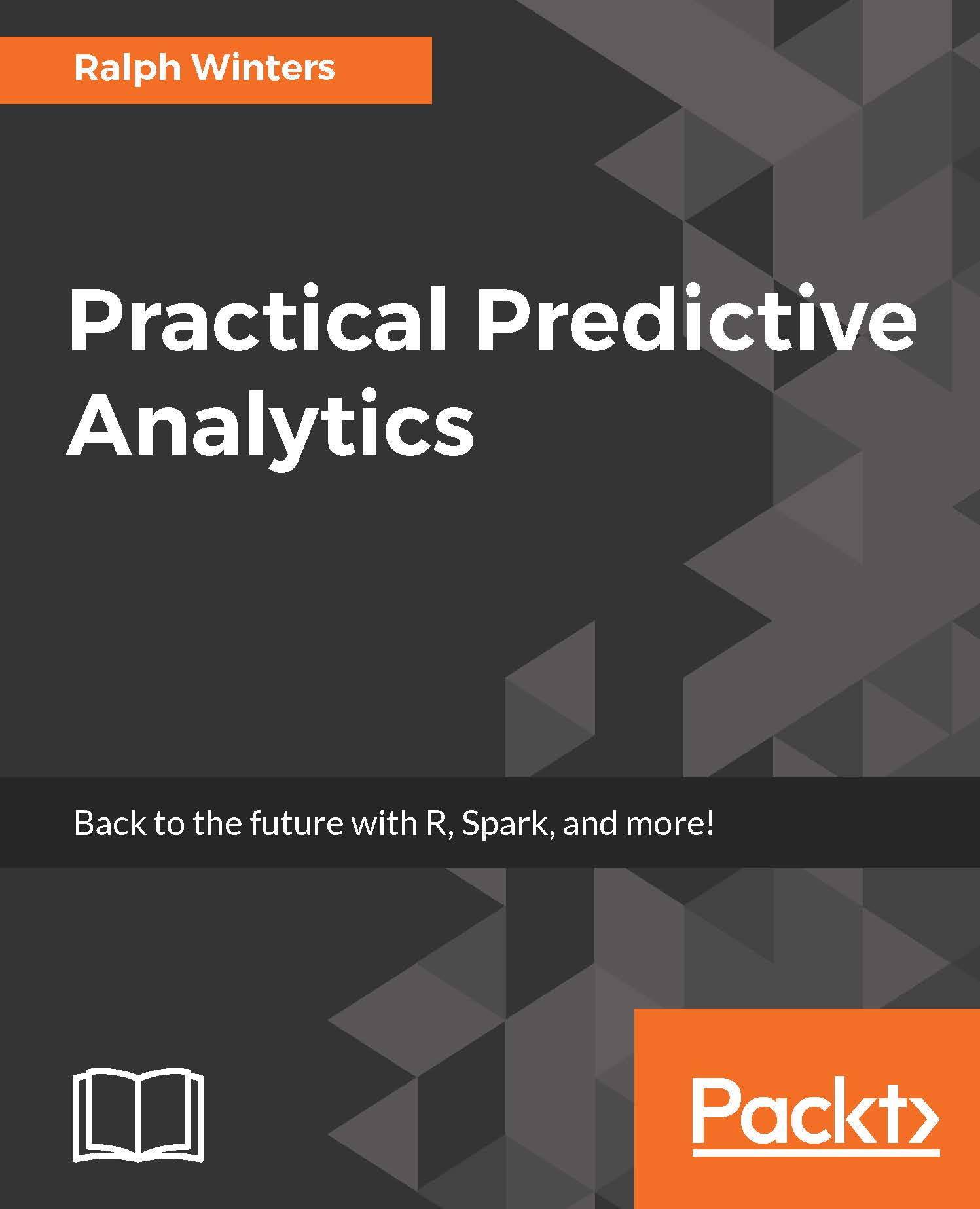
Practical Predictive Analytics

Practical Predictive Analytics: Analyse current and historical data to predict future trends using R, Spark, and more

eBook
€8.99 €32.99
Paperback
€41.99
Subscription
Free Trial
Renews at €18.99p/m

What do you get with Print?

Product feature icon Instant access to your digital eBook copy whilst your Print order is Shipped
Product feature icon Paperback book shipped to your preferred address
Product feature icon Download this book in EPUB and PDF formats
Product feature icon Access this title in our online reader with advanced features
Product feature icon DRM FREE - Read whenever, wherever and however you want
OR
Modal Close icon
Payment Processing...
tick Completed

Shipping Address

Billing Address

Shipping Methods
Table of content icon View table of contents Preview book icon Preview Book

Practical Predictive Analytics

Getting Started with Predictive Analytics

"In God we trust, all others must bring Data"

- Deming

I enjoy working and explaining predictive analytics to people because it is based upon a simple concept: predicting the probability of future events based upon historical data. Its history may date back to at least 650 BC. Some early examples include the Babylonians, who tried to predict short-term weather changes based on cloud appearances and halos: Weather Forecasting through the Ages, NASA.

Medicine also has a long history of needing to classify diseases. The Babylonian king Adad-apla-iddina decreed that medical records be collected to form the Diagnostic Handbook. Some predictions in this corpus list treatments based on the number of days the patient had been sick, and their pulse rate (Linda Miner et al., 2014). One of the first instances of bioinformatics!

In later times, specialized predictive analytics was developed at the onset of the insurance underwriting industries. This was used as a way to predict the risk associated with insuring marine vessels (https://www.lloyds.com/lloyds/about-us/history/corporate-history). At about the same time, life insurance companies began predicting the age that a person would live to in order to set the most appropriate premium rates.

Although the idea of prediction always seemed to be rooted early in the human need to understand and classify, it was not until the 20th century, and the advent of modern computing, that it really took hold.

In addition to helping the US government in the 1940s break code, Alan Turing also worked on the initial computer chess algorithms that pitted man against machine. Monte Carlo simulation methods originated as part of the Manhattan project, where mainframe computers crunched numbers for days in order to determine the probability of nuclear attacks (Computing and the Manhattan Project, n.d).

In the 1950s, Operations Research (OR) theory developed, in which one could optimize the shortest distance between two points. To this day, these techniques are used in logistics by companies such as UPS and Amazon.

Non-mathematicians have also gotten in on the act. In the 1970s, cardiologist Lee Goldman (who worked aboard a submarine) spend years developing a decision tree that did this efficiently. This helped the staff determine whether or not the submarine needed to resurface in order to help the chest pain sufferers (Gladwell, 2005)!

What many of these examples had in common was that people first made observations about events which had already occurred, and then used this information to generalize and then make decisions about might occur in the future. Along with prediction, came further understanding of cause and effect and how the various parts of the problem were interrelated. Discovery and insight came about through methodology and adhering to the scientific method.

Most importantly, they came about in order to find solutions to important, and often practical, problems of the times. That is what made them unique.

Predictive analytics are in so many industries

We have come a long way since then, and practical analytics solutions have furthered growth in so many different industries. The internet has had a profound effect on this; it has enabled every click to be stored and analyzed. More data is being collected and stored, some with very little effort, than ever before. That in itself has enabled more industries to enter predictive analytics.

Predictive Analytics in marketing

One industry that has embraced PA for quite a long time is marketing. Marketing has always been concerned with customer acquisition and retention, and has developed predictive models involving various promotional offers and customer touch points, all geared to keeping customers and acquiring new ones. This is very pronounced in certain segments of marking, such as wireless and online shopping cards, in which customers are always searching for the best deal.

Specifically, advanced analytics can help answer questions such as, If I offer a customer 10% off with free shipping, will that yield more revenue than 15% off with no free shipping? The 360-degree view of the customer has expanded the number of ways one can engage with the customer, therefore enabling marketing mix and attribution modeling to become increasingly important. Location-based devices have enabled marketing predictive applications to incorporate real-time data to issue recommendation to the customer while in the store.

Predictive Analytics in healthcare

Predictive analytics in healthcare has its roots in clinical trials, which use carefully selected samples to test the efficacy of drugs and treatments. However, healthcare has been going beyond this. With the advent of sensors, data can be incorporated into predictive analytics to monitor patients with critical illness, and to send alerts to the patient when he is at risk. Healthcare companies can now predict which individual patients will comply with courses of treatment advocated by health providers. This will send early warning signs to all parties, which will prevent future complications, as well as lower the total cost of treatment.

Predictive Analytics in other industries

Other examples can be found in just about every other industry. Here are just a few:

  • Finance:
    • Fraud detection is a huge area. Financial institutions are able to monitor client's internal and external transactions for fraud, through pattern recognition and other machine learning algorithms, and then alert a customer concerning suspicious activity. Analytics are often performed in real time. This is a big advantage, as criminals can be very sophisticated and be one step ahead of the previous analysis.
    • Wall street program trading. Trading algorithms will predict intraday highs and lows, and will decide when to buy and sell securities.
  • Sports management:
    • Sports management analytics is able to predict which sports events will yield the greatest attendance and institute variable ticket pricing based upon audience interest.
    • In baseball, a pitcher's entire game can be recorded and then digitally analyzed. Sensors can also be attached to their arm, to alert when future injury might occur.
  • Higher education:
    • Colleges can predict how many, and which kind of, students are likely to attend the next semester, and be able to plan resources accordingly. This is a challenge which is beginning to surface now, many schools may be looking at how scoring changes made to the SAT in 2016 are affecting admissions.
    • Time-based assessments of online modules can enable professors to identify students' potential problems areas, and tailor individual instruction.
  • Government:
    • Federal and State Governments have embraced the open data concept and have made more data available to the public, which has empowered Citizen Data Scientists to help solve critical social and governmental problems.
    • The potential use of data for the purpose of emergency services, traffic safety, and healthcare use is overwhelmingly positive.

Although these industries can be quite different, the goals of predictive analytics are typically implemented to increase revenue, decrease costs, or alter outcomes for the better.

Skills and roles that are important in Predictive Analytics

So what skills do you need to be successful in predictive analytics? I believe that there are three basic skills that are needed:

  • Algorithmic/statistical/programming skills: These are the actual technical skills needed to implement a technical solution to a problem. I bundle these all together since these skills are typically used in tandem. Will it be a purely statistical solution, or will there need to be a bit of programming thrown in to customize an algorithm, and clean the data? There are always multiple ways of doing the same task and it will be up to you, the predictive modeler, to determine how it is to be done.
  • Business skills: These are the skills needed for communicating thoughts and ideas among groups of the interested parties. Business and data analysts who have worked in certain industries for long periods of time, and know their business very well, are increasingly being called upon to participate in predictive analytics projects. Data science is becoming a team sport and most projects include working with others in the organization, summarizing findings, and having good presentation and documentation skills are important. You will often hear the term domain knowledge associated with this. Domain knowledge is important since it allows you to apply your particular analytics skills to the particular analytic problems of whatever business you are (or wish to) work within. Everyone business has its own nuances when it comes to solving analytic problems. If you do not have the time or inclination to learn all about the inner workings of the problem at hand yourself, partner with someone who does. That will be the start of a great team!
  • Data storage/Extract Transform and Load (ETL) skills: This can refer to specialized knowledge regarding extracting data, and storing it in a relational or non-relational NoSQL data store. Historically, these tasks were handled exclusively within a data warehouse. But now that the age of big data is upon us, specialists have emerged who understand the intricacies of data storage, and the best way to organize it.

Related job skills and terms

Along with the term predictive analytics, here are some terms that are very much related:

  • Predictive modeling: This specifically means using a mathematical/statistical model to predict the likelihood of a dependent or target variable. You may still be able to predict; however, if there is no underlying model, it is not a predictive model.
  • Artificial intelligence (AI): A broader term for how machines are able to rationalize and solve problems. AI's early days were rooted in neural networks.
  • Machine learning: A subset of AI. Specifically deals with how a machine learns automatically from data, usually to try to replicate human decision-making or to best it. At this point, everyone knows about Watson, who beat two human opponents in Jeopardy.
  • Data science: Data science encompasses predictive analytics but also adds algorithmic development via coding, and good presentation skills via visualization.
  • Data engineering: Data engineering concentrates on data extraction and data preparation processes, which allow raw data to be transformed into a form suitable for analytics. A knowledge of system architecture is important. The data engineer will typically produce the data to be used by the predictive analysts (or data scientists).
  • Data analyst/business analyst/domain expert: This is an umbrella term for someone who is well versed in the way the business at hand works, and is an invaluable person to learn from in terms of what may have meaning, and what may not.
  • Statistics: The classical form of inference, typically done via hypothesis testing. Statistics also forms the basis for the probability distributions used in machine learning, and is closely tied with predictive analytics and data science.

Predictive analytics software

Originally, predictive analytics was performed by hand, by statisticians on mainframe computers using a progression of various language such as FORTRAN. Some of these languages are still very much in use today. FORTRAN, for example, is still one of the fastest-performing languages around, and operates with very little memory. So, although it may no longer be as widespread in predictive model development as other languages, it certain can be used to implement models in a production environment.

Nowadays, there are many choices about which software to use, and many loyalists remain true to their chosen software. The reality is that for solving a specific type of predictive analytics problem, there exists a certain amount of overlap, and certainly the goal is the same. Once you get the hang of the methodologies used for predictive analytics in one software package, it should be fairly easy to translate your skills to another package.

Open source software

Open source emphasizes agile development and community sharing. Of course, open source software is free, but free must also be balanced in the context of Total Cost Of Ownership (TCO). TCO costs include everything that is factored into a softwares cost over a period of time: that not only includes the cost of the software itself, but includes training, infrastructure setup, maintenance, people costs, as well as other expenses associated with the quick upgrade and development cycles which exist in some products.

Closed source software

Closed source (or proprietary) software such as SAS and SPSS was at the forefront of predictive analytics, and has continued to this day to extend its reach beyond the traditional realm of statistics and machine learning. Closed source software emphasizes stability, better support, and security, with better memory management, which are important factors for some companies.

Peaceful coexistence

There is much debate nowadays regarding which one is better. My prediction is that they both will coexist peacefully, with one not replacing the other. Data sharing and common APIs will become more common. Each has its place within the data architecture and ecosystem that are deemed correct for a company. Each company will emphasize certain factors, and both open and closed software systems are constantly improving themselves. So, in terms of learning one or the other, it is not an either/or decision. Predictive analytics, per second does not care what software you use. Please be open to the advantages offered by both open and closed software. If you do, that will certainly open up possibilities for working for different kinds of companies and technologies

Other helpful tools

Man does not live by bread alone, so it would behave you to learn additional tools in addition to R, so as to advance your analytic skills:

  • SQL: SQL is a valuable tool to know, regardless of which language/package/environment you choose to work in. Virtually every analytics tool will have a SQL interface, and knowledge of how to optimize SQL queries will definitely speed up your productivity, especially if you are doing a lot of data extraction directly from a SQL database. Today's common thought is to do as much pre-processing as possible within the database, so if you will be doing a lot of extracting from databases such as MySQL, PostgreSQL, Oracle, or Teradata, it will be a good thing to learn how queries are optimized within their native framework.
    In the R language, there are several SQL packages that are useful for interfacing with various external databases. We will be using sqldf, which is a popular R package for interfacing with R dataframes. There are other packages that are specifically tailored for the specific database you will be working with.
  • Web extraction tools: Not every data source will originate from a data warehouse. Knowledge of APIs that extract data from the internet will be valuable to know. Some popular tools include Curl and Jsonlite.
  • Spreadsheets: Despite their problems, spreadsheets are often the fastest way to do quick data analysis and, more importantly, enable you to share your results with others! R offers several interfaces to spreadsheets but, again, learning standalone spreadsheet skills such as pivot tables and Virtual Basic for applications will give you an advantage if you work for corporations in which these skills are heavily used.
  • Data visualization tools: Data visualization tools are great for adding impact to an analysis, and for concisely encapsulating complex information. Native R visualization tools are great, but not every company will be using R. Learn some third-party visualization tools such as D3.js, Google Charts, Qlikview, or Tableau.
  • Big data, Spark, Hadoop, NoSQL database: It is becoming increasingly important to know a little bit about these technologies, at least from the viewpoint of having to extract and analyze data that resides within these frameworks. Many software packages have APIs that talk directly to Hadoop and can run predictive analytics directly within the native environment, or extract data and perform the analytics locally.

Past the basics

Given that the predictive analytics space is so huge, once you are past the basics, ask yourself what area of predictive analytics really interests you, and what you would like to specialize in. Learning all you can about everything concerning predictive analytics is good at the beginning, but ultimately you will be called upon because you are an expert in certain industries or techniques. This could be research, algorithmic development, or even managing analytics teams.

Data analytics/research

But, as general guidance, if you are involved in, or are oriented toward, data, the analytics or research portion of data science, I would suggest that you concentrate on data mining methodologies and specific data modeling techniques that are heavily prevalent in the specific industries that interest you.

For example, logistic regression is heavily used in the insurance industry, but social network analysis is not. Economic research is geared toward time series analysis, but not so much cluster analysis. Recommender engines are prevalent in online retail.

Data engineering

If you are involved more on the data engineering side, concentrate more on data cleaning, being able to integrate various data sources, and the tools needed to accomplish this.

Management

If you are a manager, concentrate on model development, testing and control, metadata, and presenting results to upper management in order to demonstrate value or return on investment.

Team data science

Of course, predictive analytics is becoming more of a team sport, rather than a solo endeavor, and the data science team is very much alive. There is a lot that has been written about the components of a data science team, much of which can be reduced to the three basic skills that I outlined earlier.

Two different ways to look at predictive analytics

Various industries interpret the goals of predictive analytics differently. For example, social science and marketing like to understand the factors which go into a model, and can sacrifice a bit of accuracy if a model can be explained well enough. On the other hand, a black box stock trading model is more interested in minimizing the number of bad trades, and at the end of the day tallies up the gains and losses, not really caring which parts of the trading algorithm worked. Accuracy is more important in the end.

Depending upon how you intend to approach a particular problem, look at how two different analytical mindsets can affect the predictive analytics process:

  1. Minimize prediction error goal: This is a very common use case for machine learning. The initial goal is to predict using the appropriate algorithms in order to minimize the prediction error. If done incorrectly, an algorithm will ultimately fail and it will need to be continually optimized to come up with the new best algorithm. If this is performed mechanically without regard to understanding the model, this will certainly result in failed outcomes. Certain models, especially over optimized ones with many variables, can have a very high prediction rate, but be unstable in a variety of ways. If one does not have an understanding of the model, it can be difficult to react to changes in the data input.
  2. Understanding model goal: This came out of the scientific method and is tied closely to the concept of hypothesis testing. This can be done in certain kinds of models, such as regression and decision trees, and is more difficult in other kinds of models such as Support Vector Machine (SVM) and neural networks. In the understanding model paradigm, understanding causation or impact becomes more important than optimizing correlations. Typically, understanding models has a lower prediction rate, but has the advantage of knowing more about the causations of the individual parts of the model, and how they are related. For example, industries that rely on understanding human behavior emphasize understanding model goals. A limitation to this orientation is that we might tend to discard results that are not immediately understood. It takes discipline to accept a model with lower prediction ability. However, you can also gain model stability

Of course, the previous examples illustrate two disparate approaches. Combination models, which use the best of both worlds, should be the ones we should strive for. Therefore, one goal for a final model is one which:

  • Has an acceptable prediction error
  • Is stable over time
  • Needs a minimum of maintenance
  • Is simple enough to understand and explain.

You will learn later that is this related to Bias/Variance tradeoff.

R

Most of the code examples in this book are written in R. As a prerequisite to this book, it is presumed that you will have some basic R knowledge, as well as some exposure to statistics. If you already know about R, you may skip this section, but I wanted to discuss it a little bit for completeness.

The R language is derived from the S language which was developed in the 1970s. However, the R language has grown beyond the original core packages to become an extremely viable environment for predictive analytics.

Although R was developed by statisticians for statisticians, it has come a long way since its early days. The strength of R comes from its package system, which allows specialized or enhanced functionality to be developed and linked to the core system.

Although the original R system was sufficient for statistics and data mining, an important goal of R was to have its system enhanced via user-written contributed packages. At the time of writing, the R system contains more than 10,000 packages. Some are of excellent quality, and some are of dubious quality. Therefore, the goal is to find the truly useful packages that add the most value.

Most, if not all, R packages in use address most common predictive analytics tasks that you will encounter. If you come across a task that does not fit into any category, the chances are good that someone in the R community has done something similar. And of course, there is always a chance that someone is developing a package to do exactly what you want it to do. That person could be eventually be you!

CRAN

The Comprehensive R Archive Network (CRAN) is a go-to site which aggregates R distributions, binaries, documentation, and packages. To get a sense of the kind of packages that could be valuable to you, check out the Task Views section maintained by CRAN here:

https://cran.r-project.org/web/views/

R installation

R installation is typically done by downloading the software directly from the Comprehensive R Archive Network (CRAN) site:

  1. Navigate to https://cran.r-project.org/.
  2. Install the version of R appropriate for your operating system. Please read any notes regarding downloading specific versions. For example, if you are a Mac user may need to have XQuartz installed in addition to R, so that some graphics can render correctly.

Alternate ways of exploring R

Although installing R directly from the CRAN site is the way most people will proceed, I wanted to mention some alternative R installation methods. These methods are often good in instances when you are not always at your computer:

  • Virtual environment: Here are a few ways to install R in the virtual environment:
    • VirtualBox or VMware: Virtual environments are good for setting up protected environments and loading preinstalled operating systems and packages. Some advantages are that they are good for isolating testing areas, and when you do not wish to take up additional space on your own machine.
    • Docker: Docker resembles a virtual machine, but is a bit more lightweight since it does not emulate an entire operating system, but emulates only the needed processes.
  • Cloud-based: Here are a few methods to install R in the cloud-based environment. Cloud based environments as perfect for working in situations when you are not working directly on your computer:
    • AWS/Azure: These are three environments which are very popular. Reasons for using cloud based environments are similar to the reasons given for virtual environment, but also have some additional advantages: such as the additional capability to run with very large datasets and with more memory. All of the previously mentioned require a subscription service to use, however free tiers are offered to get started. We will explore Databricks in depth in later chapters, when we learn about predictive analytics using R and SparkR
  • Web-based: Web-based platforms are good for learning R and for trying out quick programs and analysis. R-Fiddle is a good choice, however there are other including: R-Web, Jupyter, Tutorialspoint, and Anaconda Cloud.
  • Command line: R can be run purely from a command line. When R is run this way, it is usually coupled with other Linux tools such as curl, grep, awk, and various customized text editors, such as Emacs Speaks Statistics (ESS). Often R is run this way in production mode, when processes need to be automated and scheduled directly via the operating system

How is a predictive analytics project organized?

After you install R on your own machine, I would give some thought to how you want to organize your data, code, documentation, and so on. There will probably be many different kinds of projects that you will need to set up, ranging from exploratory analysis to full production-grade implementations. However, most projects will be somewhere in the middle, that is, those projects that ask a specific question or a series of related questions. Whatever their purpose, each project you will work on will deserve its own project folder or directory.

Some important points to remember about constructing projects:

  • It is never a good idea to boil the ocean, or try to answer too many questions at once. Remember, predictive analytics is an iterative process.
  • Another trap that people fall into is not having their project reproducible. Nothing is worse than to develop some analytics on a set of data, and then backtrack, and oops! different results.
  • When organizing code, try to write code as building block, which can be reusable. For R, write code liberally as functions.
  • Assume that anything concerning requirements, data, and outputs will change, and be prepared.
  • Considering the dynamic nature of the R language. Changes in versions, and packages could all change your analysis in various ways, so it is important to keep code and data in sync, by using separate folders for the different levels of code, data, and so on or by using version management packages such as subversion, git, or cvs.

Once you have considered all of the preceding points, physically set up your folder environment.

Setting up your project and subfolders

We will start by creating folders for our environment. Often projects start with three subfolders which roughly correspond to:

  • Data source
  • Code-generated outputs
  • The code itself (in this case, R)

There may be more in certain cases, but lets keep it simple:

  • First, decide where you will be housing your projects. Then create a sub-directory and name it PracticalPredictiveAnalytics. For this example, we will create the directory under Windows drive C.
  • Create three subdirectories under this project: Data, Outputs, and R:
    • The R directory will hold all of our data prep code, algorithms, and so on.
    • The Data directory will contain our raw data sources that will typically be read in by our programs.
    • The Outputs directory will contain anything generated by the code. That can include plots, tables, listings, and output from the log.

Here is an example of how the structure will look after you have created the folders:

GUIs

R, like many languages and knowledge discovery systems, started from the command line. However, predictive analysts tend to prefer Graphic User Interfaces (GUIs), and there are many choices available for each of the three different operating systems (Mac, Windows, and Linux). Each of them has its strengths and weaknesses, and of course there is always the question of preference.

Memory is always a consideration with R, and if that is of critical concern to you, you might want to go with a simpler GUI, such as the one built in with R.

If you want full control, and you want to add some productive tools, you could choose RStudio, which is a full-blown GUI and allows you to implement version control repositories, and has nice features such as code completion.

R Commander (Rcmdr), and Rattle unique features are that they offer menus that allow guided point and click commands for common statistical and data mining tasks. They are always both code generators. This is a way to start when learning R, since you can use the menus to accomplish the tasks, and then by looking at the way the code was generated for each particular task. If you are interested in predictive analytics using Rattle, I have written a nice tutorial on using R with Rattle which can be found in the tutorial section of Practical Predictive Analytics and Decisioning Systems for Medicine, which is referenced at the end of this chapter.

Both RCmdr and RStudio offer GUIs that are compatible with the Windows, Apple, and Linux operator systems, so those are the ones I will use to demonstrate examples in this book. But bear in mind that they are only user interfaces, and not R proper, so it should be easy enough to paste code examples into other GUIs and decide for yourself which ones you like.

Getting started with RStudio

After R installation has completed, point your browser to the download section found through the RStudio web site (https://www.rstudio.com/) and install the RStudio executable appropriate for your operating system:

  • Click the RStudio icon to bring up the program.
  • The program initially starts with three tiled window panes, as shown in the following screenshot. If the layout does not correspond exactly to what is shown, the next section will show you how to rearrange the layout to correspond with the examples shown in this chapter:

Rearranging the layout to correspond with the examples

To rearrange the layout, see the following steps:

  1. Select Tools | Global Options | Pane Layout from the top navigation bar.
  2. Select the drop-down arrow in each of the four quadrants, and change the title of each pane to what is shown in the following diagram.
    • Make sure that Environment | History | Files | Plots and Help are selected for the upper left pane
    • Make sure that Viewer is selected for the bottom left pane.
    • Select Console for the bottom right pane
    • Select Source for the upper right pane
  3. Click OK.

After the changes are applied the layout should more closely match the layout previously shown . However, it may not match exactly. A lot will depend upon the version of RStudio that you are using as well as the packages you may have already installed.

Brief description of some important panes

  • The Source pane will be used to code and save your programs. Once code is created you can use File | Save to save your work to an external file, and File |Open to retrieve the saved code.
If you are installing RStudio for the first time nothing may be shown as the fourth pane. However, as you create new programs (as we will later in this chapter), it will appear in the upper right quadrant.
  • The Console pane provides important feedback and information about your program after it has been run. It will show you any syntax or error messages that have occurred. It is always a best practice to examine the console to make sure you are getting the results you expect, and make sure the console is clear of errors. The console is also the place that you will see a lots of output which has been created from your programs.
  • We will rely heavily on the View pane. This pane displays formatted output which is run by using the R View command.
  • The Environment | History | Plots pane is sort of a catch-all pane which changes functions depending upon what which tabs have been selected via the pane layout dialogue. For example, all plots issued by R command are displayed under the Plots tab. Help is always a click away by selecting the Help tab. There is also a useful tab called Packages which will automatically load a package, when a particular package is checked.

Creating a new project

Once you are set with your layout, proceed to create a new project by following these steps:

Create a new project by following these steps:

  1. Identify the menu bar, above the icons at the top left of the screen.
  2. Click File and then New Project
  3. At the next screen select Existing Directory:
  1. The following screen will appear:
  1. The Project working directory is initial populated with a tilde (~). This means that the project will be created in the directory you are currently in.
  2. To specify the directory first select Browse, and then navigate to the PracticalPredictiveAnalytics folder you created in the previous steps.
  3. When the Choose Directory dialog box appear, select this directory using the Select Folder button.
  4. After selecting the directory, the following should appear (Windows only):
  1. To finalize creating the project, Select the Create Project button. Rstudio will then switch to the new project you have just created.

All screen panes will then appear as blank (except for the log), and the title bar at the top left of the screen will show the path to the project.

To verify that the R, outputs, and data directories are contained within the project, select File, and then File Open from the top menu bar. The three folders should appear, as indicated as follows:

Once you have verified this, cancel the Open File dialogue, and return to RStudio main screen.

The R console

Now that we have created a project, let us take a look at the R Console window. Click on the window marked Console. All console commands are issued by typing your command following the command prompt >, and then pressing Enter. I will just illustrate three commands that will help you answer the questions "Which project am I on?", and "What files do I have in my folders?"

  1. getwd(): The getwd() command is very important since it will always tell you which directory you are in. Since we just created a new project, we expect that we will be pointing to the directory we just created, right?
    To double check, switch over to the console, issue the getwd() command, and then press Enter. That should echo back the current working directory:
  1. dir(): The dir() command will give you a list of all files in the current working directory. In our case, it is simply the names of the three directories you have just created. However, typically may see many files, usually corresponding to the type of directory you are in (.R for source files, .dat, .csv for data files, and so on):
  1. setwd(): Sometimes you will need to switch directories within the same project or even to another project. The command you will use is setwd(). You will supply the directory that you want to switch to, all contained within the parentheses.
    Here is an example which will switch to the sub-directory which will house the R code. This particular example supplies the entire path as the directory destination. Since you are already in the PracticalPredictiveAnalytics directory, you can also use setwd(“R”) which accomplishes the same thing:
        > setwd("C:/PracticalPredictiveAnalytics/R")

To verify that it has changed, issue the getwd() command again:

        > getwd()
[1] "C:/PracticalPredictiveAnalytics/R"

I suggest using getwd() and setwd() liberally, especially if you are working on multiple projects, and want to avoid reading or writing the wrong files.

The source window

The Source window is where all of your R code appears. It is also where you will be probably spending most of your time. You can have several script windows open, all at once.

Creating a new script

To create a new script select File | New File | R Script from the top navigation bar. A new blank script window will appear with the name Untitled1.

Once it appears you can start entering code!

Our first predictive model

Now that all of the preliminary things are out of the way, we will code our first extremely simple predictive model. There will be two scripts written to accomplish this.

Our first R script is not a predictive model (yet), but it is a preliminary program which will view and plot some data. The dataset we will use is already built into the R package system, and is not necessary to load externally. For quickly illustrating techniques, I will sometimes use sample data contained within specific R packages themselves in order to demonstrate ideas, rather than pulling data in from an external file.

In this case our data will be pulled from the datasets package, which is loaded by default at startup.

  • Paste the following code into the Untitled1 scripts that was just created. Dont worry about what each line means yet. I will cover the specific lines after the code is executed:
        require(graphics)
data(women)
head(women)
View(women)
plot(women$height,women$weight)
  • Within the code pane, you will see a menu bar right beneath the Untitled1 tab. It should look something like this:
  • To execute the code, Click the Source icon. The display should then change to the following diagram:

Notice from the preceding picture that three things have changed:

  1. Output has been written to the Console pane.
  2. The View pane has popped up which contains a two column table.
  3. Additionally, a plot will appear in the Plot pane.

Code description

Here are some more details on what the code has accomplished:

  • Line 1 of the code contains the function require, which is just a way of saying that R needs a specific package to run. In this case require(graphics) specifies that the graphics package is needed for the analysis, and it will load it into memory. If it is not available, you will get an error message. However, graphics is a base package and should be available.
  • Line 2 of the code loads the Women data object into memory using the data(women) function.
  • Lines 3-5 of the code display the raw data in three different ways:
    • View(women): This will visually display the DataFrame. Although this is part of the actual R script, viewing a DataFrame is a very common task, and is often issued directly as a command via the R Console. As you can see in the previous figure , the Women dataframe has 15 rows, and 2 columns named height and weight.
    • plot(women$height,women$weight): This uses the native R plot function, which plots the values of the two variables against each other. It is usually the first step one does to begin to understand the relationship between two variables. As you can see, the relationship is very linear.
    • head(women): This displays the first N rows of the Women dataframe to the console. If you want no more than a certain number of rows, add that as a second argument of the function. For example, Head(women,99) will display up to 99 rows in the console. The tail() function works similarly, but displays the last rows of data.
The utils:View(women) function can also be shortened to just View(women). I have added the prefix utils:: to indicate that the View() function is part of the utils package. There is generally no reason to add the prefix unless there is a function name conflict. This can happen when you have identically named functions sourced from two different packages which are loaded in memory. We will see these kind of function name conflicts in later chapters. But it is always safe to prefix a function name with the name of the package that it comes from.

Saving the script

To save this script, navigate to the top navigation menu bar and select File | Save. When the file selector appears navigate to the PracticalPredictiveAnalytics/R folder that was created, and name the file Chapter1_DataSource. Then select Save.

Your second script

Our second R script is a simple two variable regression model which predicts womens height based upon weight.

Begin by creating another R script by selecting File | New File | R Script from the top navigation bar. If you create new scripts via File | New File | R Script often enough you might get Click Fatigue (uses three clicks), so you can also save a click by selecting the icon in the top left with the + sign:

Whichever way you choose , a new blank script window will appear with the name Untitled2.

Now paste the following code into the new script window:

require(graphics)
data(women)
lm_output <- lm(women$height ~ women$weight)
summary(lm_output)
prediction <- predict(lm_output)
error <- women$height-prediction
plot(women$height,error)

Press the Source icon to run the entire code. The display will change to something similar to what is displayed as follows:

Code description

Here are some notes and explanations for the script code that you have just run:

  • lm() function: This function runs a simple linear regression using the lm() function. This function predicts women's height based upon the value of their weight. In statistical parlance, you will be regressing height on weight. The line of code which accomplishes this is:
        lm_output <- lm(women$height ~ women$weight) 
  • There are two operations that you will become very familiar with when running predictive models in R:
    • The ~ operator: Also called the tilde, this is a shorthand way for separating what you want to predict, with what you are using to predict. This is an expression in formula syntax. What you are predicting (the dependent or target variable) is usually on the left side of the formula, and the predictors (independent variables, features) are on the right side. In order to improve readability, the independent variable (weight) and dependent variable (height) are specified using $ notation which specifies the object name, $, and then the dataframe column. So womens height is referenced as women$height and womens weight is referenced as women$weight. Alternatively, you can use the attach command, and then refer to these columns only by specifying the names height and weight. For example, the following code would achieve the same results:
                      attach(women)
lm_output <- lm(height ~ weight)
    • The <- operator: Also called the assignment operator. This common statement assigns whatever expressions are evaluated on the right side of the assignment operator to the object specified on the left side of the operator. This will always create or replace a new object that you can further display or manipulate. In this case, we will be creating a new object called lm_output, which is created using the function lm(), which creates a linear model based on the formula contained within the parentheses.
Note that the execution of this line does not produce any displayed output. You can see whether the line was executed by checking the console. If there is any problem with running the line (or any line for that matter), you will see an error message in the console.
  • summary(lm_output): The following statement displays some important summary information about the object lm_output and writes to output to the R Console as pictured previously:
        summary(lm_output) 
  • The results will appear in the Console window as pictured in the previous figure. Just to keep thing a little bit simpler for now, I will just show the first few lines of the output, and underline what you should be looking at. Do not be discouraged by the amount of output produced.
  • Look at the lines marked Intercept and women$weight which appear under the coefficients line in the console.
        Coefficients:
Estimate Std. Error t value Pr(>|t|)
(Intercept) 25.723456 1.043746 24.64 2.68e-12 ***
women$weight 0.287249 0.007588 37.85 1.09e-14 ***
  • The Estimate column illustrates the linear regression formula needed to derive height from weight. We can actually use these numbers along with a calculator to determine the prediction ourselves. For our example the output tells us that we should perform the following steps for all of the observations in our dataframe in order to obtain the prediction for height. We will obviously not want to do all of the observations (R will do that via the following predict() function), but we will illustrate the calculation for 1 data point:
    • Take the weight value for each observation. Lets take the weight of the first woman which is 115 lbs.
    • Then,multiply weight by 0.2872 . That is the number that is listed under Estimate for womens$weight. Multiplying 115 lbs. by 0.2872 yield 33.028
    • Then add 25.7235 which is the estimate of the (intercept) row. That will yield a prediction of 58.75 inches.
  • If you do not have a calculator handy, the calculation is easily done in calculator mode via the R Console, by typing the following:

The predict function

To predict the value for all of the values we will use a function called predict(). This function reads each input (independent) variable and then predicts a target (dependent) variable based on the linear regression equation. In the code we have assigned the output of this function to a new object named prediction.

Switch over to the console area, and type prediction, then Enter, to see the predicted values for the 15 women. The following should appear in the console.

> prediction
1 2 3 4 5 6 7
58.75712 59.33162 60.19336 61.05511 61.91686 62.77861 63.64035
8 9 10 11 12 13 14
64.50210 65.65110 66.51285 67.66184 68.81084 69.95984 71.39608
15
72.83233

Notice that the value of the first prediction is very close to what you just calculated by hand. The difference is due to rounding error.

Examining the prediction errors

Another R object produced by our linear regression is the error object. The error object is a vector that was computed by taking the difference between the predicted value of height and the actual height. These values are also known as the residual errors, or just residuals.

error <- women$height-prediction

Since the error object is a vector, you cannot use the nrow() function to get its size. But you can use the length() function:

>length(error)
[1] 15

In all of the previous cases, the counts all total 15, so all is good. If we want to see the raw data, predictions, and the prediction errors for all of the data, we can use the cbind() function (Column bind) to concatenate all three of those values, and display as a simple table.

At the console enter the follow cbind command:

> cbind(height=women$height,PredictedHeight=prediction,ErrorInPrediction=error)
height PredictedHeight ErrorInPrediction
1 58 58.75712 -0.75711680
2 59 59.33162 -0.33161526
3 60 60.19336 -0.19336294
4 61 61.05511 -0.05511062
5 62 61.91686 0.08314170
6 63 62.77861 0.22139402
7 64 63.64035 0.35964634
8 65 64.50210 0.49789866
9 66 65.65110 0.34890175
10 67 66.51285 0.48715407
11 68 67.66184 0.33815716
12 69 68.81084 0.18916026
13 70 69.95984 0.04016335
14 71 71.39608 -0.39608278
15 72 72.83233 -0.83232892

From the preceding output, we can see that there are a total 15 predictions. If you compare the ErrorInPrediction with the error plot shown previously, you can see that for this very simple model, the prediction errors are much larger for extreme values in height (shaded values).

Just to verify that we have one for each of our original observations we will use the nrow() function to count the number of rows.

At the command prompt in the console area, enter the command:

nrow(women)

The following should appear:

>nrow(women)
[1] 15

Refer back to the seventh line of code in the original script: plot(women$height,error) plots the predicted height versus the errors. It shows how much the prediction was off from the original value. You can see that the errors show a non-random pattern.

After you are done, save the file using File | File Save, navigate to the PracticalPredictiveAnalytics/R folder that was created, and name it Chapter1_LinearRegression.

R packages

An R package extends the functionality of basic R. Base R, by itself, is very capable, and you can do an incredible amount of analytics without adding any additional packages. However adding a package may be beneficial if it adds a functionality which does not exist in base R, improves or builds upon an existing functionality, or just makes something that you can already do easier.

For example, there are no built in packages in base R which enable you to perform certain types of machine learning (such as Random Forests). As a result, you need to search for an add on package which performs this functionality. Fortunately you are covered. There are many packages available which implement this algorithm.

Bear in mind that there are always new packages coming out. I tend to favor packages which have been on CRAN for a long time and have large user base. When installing something new, I will try to reference the results against other packages which do similar things. Speed is another reason to consider adopting a new package.

The stargazer package

For an example of a package which can just make life easier, first lets consider the output produced by running a summary function on the regression results, as we did previously. You can run it again if you wish.

summary(lm_output)

The amount of statistical information output by the summary() function can be overwhelming to the initiated. This is not only related to the amount of output, but the formatting. That is why I did not show the entire output in the previous example.

One way to make output easier to look at is to first reduce the amount of output that is presented, and then reformat it so it is easier on the eyes.

To accomplish this, we can utilize a package called stargazer, which will reformat the large volume of output produced by summary() function and simplify the presentations. Stargazer excels at reformatting the output of many regression models, and displaying the results as HTML, PDF, Latex, or as simple formatted text. By default, it will show you the most important statistical output for various models, and you can always specify the types of statistical output that you want to see.

To obtain more information on the stargazer package you can first go to CRAN, and search for documentation about stargazer package, and/or you can use the R help system:

IF you already have installed stargazer you can use the following command:

packageDescription("stargazer")

If you havent installed the package, information about stargazer, (or other packages) can also be found using R specific internet searches:

RSiteSearch("stargazer")

If you like searching for documentation within R, you can obtain more information about the R help system at:

https://www.r-project.org/help.html

Installing stargazer package

Now, on to installing stargazer:

  • First create a new R script (File | New File | R Script).
  • Enter the following lines and then select Source from the menu bar in the code pane, which will submit the entire script:
        install.packages("stargazer") 
library(stargazer)
stargazer(lm_output, , type="text")

After the script has been run, the following should appear in the Console:

Code description

Here is a line by line description of the code which you have just run:

  • install.packages("stargazer"): The line will install the package to the default package directory on your machine. If you will be rerunning this code again, you can comment out this line, since the package will have already be installed in your R repository.
  • library(stargazer): Installing a package does not make the package automatically available. You need to run a library (or require()) function in order to actually load the stargazer package.
  • stargazer(lm_output, , type="text"): This line will take the output object lm_output, that was created in the first script, condense the output, and write it out to the console in a simpler, more readable format. There are many other options in the stargazer library, which will format the output as HTML, or Latex.

Please refer to the reference manual at https://cran.r-project.org/web/packages/stargazer/index.html for more information.

The reformatted results will appear in the R Console. As you can see, the output written to the console is much cleaner and easier to read.

Saving your work

After you are done, select File | File Save from the menu bar.

Then navigate to the PracticalPredictiveAnalytics/Outputs folder that was created, and name it Chapter1_LinearRegressionOutput. Press Save.

References

Summary

In this chapter, we have learned a little about what predictive analytics is and how they can be used in various industries. We learned some things about data, and how they can be organized in projects. Finally, we installed RStudio, ran a simple linear regression, and installed and ran our first package. We learned that it is always good practice to examine data after it has been loaded into memory, and a lot can be learned from simply displaying and plotting the data.

In the next chapter, we will discuss the overall predictive modeling process itself, introduce some key model packages using R, and provide some guidance on avoiding some predictive modeling pitfalls.

Left arrow icon Right arrow icon
Download code icon Download Code

Key benefits

  • A unique book that centers around develop six key practical skills needed to develop and implement predictive analytics
  • Apply the principles and techniques of predictive analytics to effectively interpret big data
  • Solve real-world analytical problems with the help of practical case studies and real-world scenarios taken from the world of healthcare, marketing, and other business domains

Description

This is the go-to book for anyone interested in the steps needed to develop predictive analytics solutions with examples from the world of marketing, healthcare, and retail. We'll get started with a brief history of predictive analytics and learn about different roles and functions people play within a predictive analytics project. Then, we will learn about various ways of installing R along with their pros and cons, combined with a step-by-step installation of RStudio, and a description of the best practices for organizing your projects. On completing the installation, we will begin to acquire the skills necessary to input, clean, and prepare your data for modeling. We will learn the six specific steps needed to implement and successfully deploy a predictive model starting from asking the right questions through model development and ending with deploying your predictive model into production. We will learn why collaboration is important and how agile iterative modeling cycles can increase your chances of developing and deploying the best successful model. We will continue your journey in the cloud by extending your skill set by learning about Databricks and SparkR, which allow you to develop predictive models on vast gigabytes of data.

Who is this book for?

This book is for those with a mathematical/statistics background who wish to understand the concepts, techniques, and implementation of predictive analytics to resolve complex analytical issues. Basic familiarity with a programming language of R is expected.

What you will learn

  • Master the core predictive analytics algorithm which are used today in business
  • Learn to implement the six steps for a successful analytics project
  • Classify the right algorithm for your requirements
  • Use and apply predictive analytics to research problems in healthcare
  • Implement predictive analytics to retain and acquire your customers
  • Use text mining to understand unstructured data
  • Develop models on your own PC or in Spark/Hadoop environments
  • Implement predictive analytics products for customers
Estimated delivery fee Deliver to Slovenia

Premium delivery 7 - 10 business days

€25.95
(Includes tracking information)

Product Details

Country selected
Publication date, Length, Edition, Language, ISBN-13
Publication date : Jun 30, 2017
Length: 576 pages
Edition : 1st
Language : English
ISBN-13 : 9781785886188
Category :
Languages :
Tools :

What do you get with Print?

Product feature icon Instant access to your digital eBook copy whilst your Print order is Shipped
Product feature icon Paperback book shipped to your preferred address
Product feature icon Download this book in EPUB and PDF formats
Product feature icon Access this title in our online reader with advanced features
Product feature icon DRM FREE - Read whenever, wherever and however you want
OR
Modal Close icon
Payment Processing...
tick Completed

Shipping Address

Billing Address

Shipping Methods
Estimated delivery fee Deliver to Slovenia

Premium delivery 7 - 10 business days

€25.95
(Includes tracking information)

Product Details

Publication date : Jun 30, 2017
Length: 576 pages
Edition : 1st
Language : English
ISBN-13 : 9781785886188
Category :
Languages :
Tools :

Packt Subscriptions

See our plans and pricing
Modal Close icon
€18.99 billed monthly
Feature tick icon Unlimited access to Packt's library of 7,000+ practical books and videos
Feature tick icon Constantly refreshed with 50+ new titles a month
Feature tick icon Exclusive Early access to books as they're written
Feature tick icon Solve problems while you work with advanced search and reference features
Feature tick icon Offline reading on the mobile app
Feature tick icon Simple pricing, no contract
€189.99 billed annually
Feature tick icon Unlimited access to Packt's library of 7,000+ practical books and videos
Feature tick icon Constantly refreshed with 50+ new titles a month
Feature tick icon Exclusive Early access to books as they're written
Feature tick icon Solve problems while you work with advanced search and reference features
Feature tick icon Offline reading on the mobile app
Feature tick icon Choose a DRM-free eBook or Video every month to keep
Feature tick icon PLUS own as many other DRM-free eBooks or Videos as you like for just €5 each
Feature tick icon Exclusive print discounts
€264.99 billed in 18 months
Feature tick icon Unlimited access to Packt's library of 7,000+ practical books and videos
Feature tick icon Constantly refreshed with 50+ new titles a month
Feature tick icon Exclusive Early access to books as they're written
Feature tick icon Solve problems while you work with advanced search and reference features
Feature tick icon Offline reading on the mobile app
Feature tick icon Choose a DRM-free eBook or Video every month to keep
Feature tick icon PLUS own as many other DRM-free eBooks or Videos as you like for just €5 each
Feature tick icon Exclusive print discounts

Frequently bought together


Stars icon
Total 120.97
Statistics for Machine Learning
€41.99
Practical Predictive Analytics
€41.99
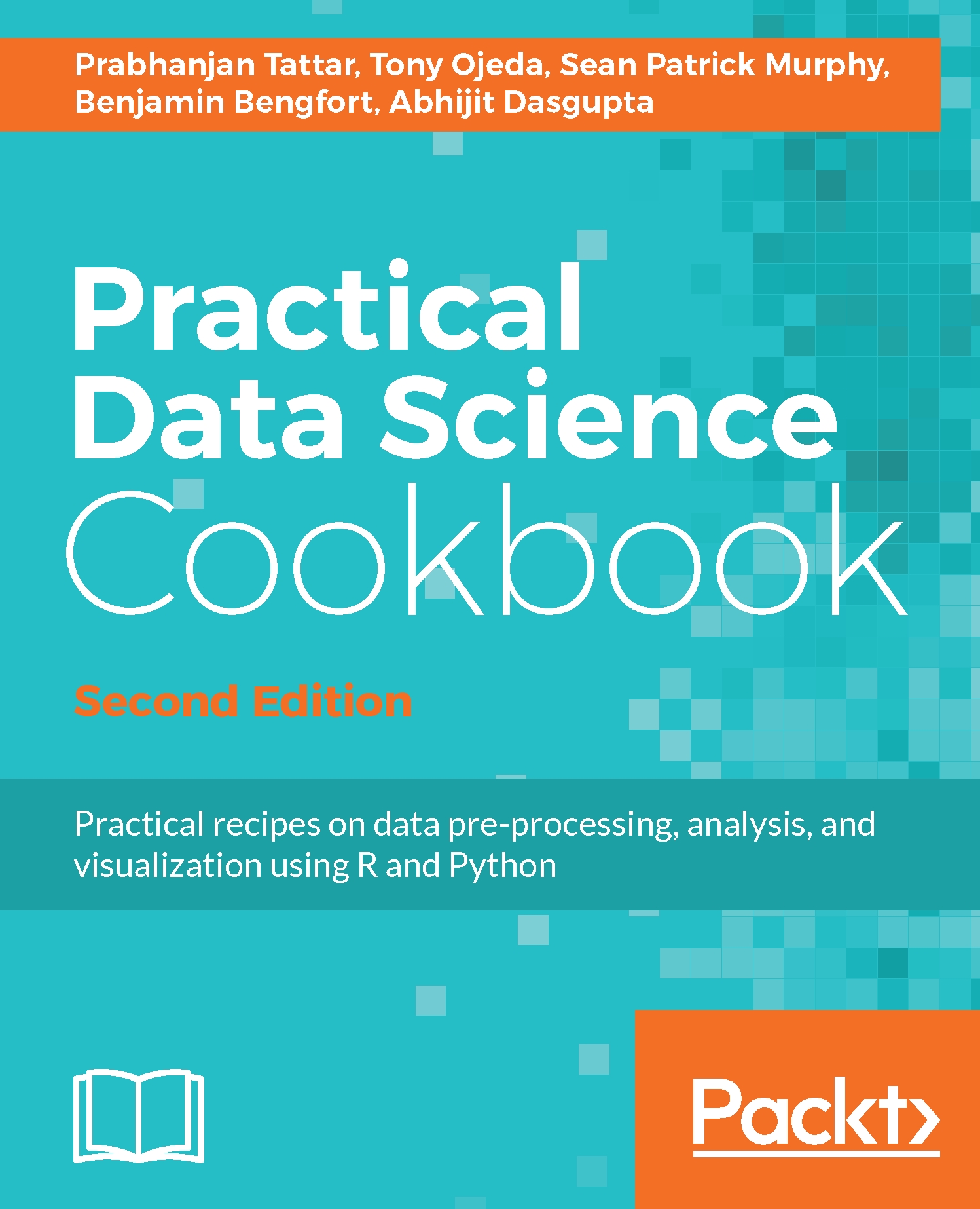
Practical Data Science Cookbook, Second Edition
€36.99
Total 120.97 Stars icon
Banner background image

Table of Contents

12 Chapters
Getting Started with Predictive Analytics Chevron down icon Chevron up icon
The Modeling Process Chevron down icon Chevron up icon
Inputting and Exploring Data Chevron down icon Chevron up icon
Introduction to Regression Algorithms Chevron down icon Chevron up icon
Introduction to Decision Trees, Clustering, and SVM Chevron down icon Chevron up icon
Using Survival Analysis to Predict and Analyze Customer Churn Chevron down icon Chevron up icon
Using Market Basket Analysis as a Recommender Engine Chevron down icon Chevron up icon
Exploring Health Care Enrollment Data as a Time Series Chevron down icon Chevron up icon
Introduction to Spark Using R Chevron down icon Chevron up icon
Exploring Large Datasets Using Spark Chevron down icon Chevron up icon
Spark Machine Learning - Regression and Cluster Models Chevron down icon Chevron up icon
Spark Models – Rule-Based Learning Chevron down icon Chevron up icon
Get free access to Packt library with over 7500+ books and video courses for 7 days!
Start Free Trial

FAQs

What is the delivery time and cost of print book? Chevron down icon Chevron up icon

Shipping Details

USA:

'

Economy: Delivery to most addresses in the US within 10-15 business days

Premium: Trackable Delivery to most addresses in the US within 3-8 business days

UK:

Economy: Delivery to most addresses in the U.K. within 7-9 business days.
Shipments are not trackable

Premium: Trackable delivery to most addresses in the U.K. within 3-4 business days!
Add one extra business day for deliveries to Northern Ireland and Scottish Highlands and islands

EU:

Premium: Trackable delivery to most EU destinations within 4-9 business days.

Australia:

Economy: Can deliver to P. O. Boxes and private residences.
Trackable service with delivery to addresses in Australia only.
Delivery time ranges from 7-9 business days for VIC and 8-10 business days for Interstate metro
Delivery time is up to 15 business days for remote areas of WA, NT & QLD.

Premium: Delivery to addresses in Australia only
Trackable delivery to most P. O. Boxes and private residences in Australia within 4-5 days based on the distance to a destination following dispatch.

India:

Premium: Delivery to most Indian addresses within 5-6 business days

Rest of the World:

Premium: Countries in the American continent: Trackable delivery to most countries within 4-7 business days

Asia:

Premium: Delivery to most Asian addresses within 5-9 business days

Disclaimer:
All orders received before 5 PM U.K time would start printing from the next business day. So the estimated delivery times start from the next day as well. Orders received after 5 PM U.K time (in our internal systems) on a business day or anytime on the weekend will begin printing the second to next business day. For example, an order placed at 11 AM today will begin printing tomorrow, whereas an order placed at 9 PM tonight will begin printing the day after tomorrow.


Unfortunately, due to several restrictions, we are unable to ship to the following countries:

  1. Afghanistan
  2. American Samoa
  3. Belarus
  4. Brunei Darussalam
  5. Central African Republic
  6. The Democratic Republic of Congo
  7. Eritrea
  8. Guinea-bissau
  9. Iran
  10. Lebanon
  11. Libiya Arab Jamahriya
  12. Somalia
  13. Sudan
  14. Russian Federation
  15. Syrian Arab Republic
  16. Ukraine
  17. Venezuela
What is custom duty/charge? Chevron down icon Chevron up icon

Customs duty are charges levied on goods when they cross international borders. It is a tax that is imposed on imported goods. These duties are charged by special authorities and bodies created by local governments and are meant to protect local industries, economies, and businesses.

Do I have to pay customs charges for the print book order? Chevron down icon Chevron up icon

The orders shipped to the countries that are listed under EU27 will not bear custom charges. They are paid by Packt as part of the order.

List of EU27 countries: www.gov.uk/eu-eea:

A custom duty or localized taxes may be applicable on the shipment and would be charged by the recipient country outside of the EU27 which should be paid by the customer and these duties are not included in the shipping charges been charged on the order.

How do I know my custom duty charges? Chevron down icon Chevron up icon

The amount of duty payable varies greatly depending on the imported goods, the country of origin and several other factors like the total invoice amount or dimensions like weight, and other such criteria applicable in your country.

For example:

  • If you live in Mexico, and the declared value of your ordered items is over $ 50, for you to receive a package, you will have to pay additional import tax of 19% which will be $ 9.50 to the courier service.
  • Whereas if you live in Turkey, and the declared value of your ordered items is over € 22, for you to receive a package, you will have to pay additional import tax of 18% which will be € 3.96 to the courier service.
How can I cancel my order? Chevron down icon Chevron up icon

Cancellation Policy for Published Printed Books:

You can cancel any order within 1 hour of placing the order. Simply contact customercare@packt.com with your order details or payment transaction id. If your order has already started the shipment process, we will do our best to stop it. However, if it is already on the way to you then when you receive it, you can contact us at customercare@packt.com using the returns and refund process.

Please understand that Packt Publishing cannot provide refunds or cancel any order except for the cases described in our Return Policy (i.e. Packt Publishing agrees to replace your printed book because it arrives damaged or material defect in book), Packt Publishing will not accept returns.

What is your returns and refunds policy? Chevron down icon Chevron up icon

Return Policy:

We want you to be happy with your purchase from Packtpub.com. We will not hassle you with returning print books to us. If the print book you receive from us is incorrect, damaged, doesn't work or is unacceptably late, please contact Customer Relations Team on customercare@packt.com with the order number and issue details as explained below:

  1. If you ordered (eBook, Video or Print Book) incorrectly or accidentally, please contact Customer Relations Team on customercare@packt.com within one hour of placing the order and we will replace/refund you the item cost.
  2. Sadly, if your eBook or Video file is faulty or a fault occurs during the eBook or Video being made available to you, i.e. during download then you should contact Customer Relations Team within 14 days of purchase on customercare@packt.com who will be able to resolve this issue for you.
  3. You will have a choice of replacement or refund of the problem items.(damaged, defective or incorrect)
  4. Once Customer Care Team confirms that you will be refunded, you should receive the refund within 10 to 12 working days.
  5. If you are only requesting a refund of one book from a multiple order, then we will refund you the appropriate single item.
  6. Where the items were shipped under a free shipping offer, there will be no shipping costs to refund.

On the off chance your printed book arrives damaged, with book material defect, contact our Customer Relation Team on customercare@packt.com within 14 days of receipt of the book with appropriate evidence of damage and we will work with you to secure a replacement copy, if necessary. Please note that each printed book you order from us is individually made by Packt's professional book-printing partner which is on a print-on-demand basis.

What tax is charged? Chevron down icon Chevron up icon

Currently, no tax is charged on the purchase of any print book (subject to change based on the laws and regulations). A localized VAT fee is charged only to our European and UK customers on eBooks, Video and subscriptions that they buy. GST is charged to Indian customers for eBooks and video purchases.

What payment methods can I use? Chevron down icon Chevron up icon

You can pay with the following card types:

  1. Visa Debit
  2. Visa Credit
  3. MasterCard
  4. PayPal
What is the delivery time and cost of print books? Chevron down icon Chevron up icon

Shipping Details

USA:

'

Economy: Delivery to most addresses in the US within 10-15 business days

Premium: Trackable Delivery to most addresses in the US within 3-8 business days

UK:

Economy: Delivery to most addresses in the U.K. within 7-9 business days.
Shipments are not trackable

Premium: Trackable delivery to most addresses in the U.K. within 3-4 business days!
Add one extra business day for deliveries to Northern Ireland and Scottish Highlands and islands

EU:

Premium: Trackable delivery to most EU destinations within 4-9 business days.

Australia:

Economy: Can deliver to P. O. Boxes and private residences.
Trackable service with delivery to addresses in Australia only.
Delivery time ranges from 7-9 business days for VIC and 8-10 business days for Interstate metro
Delivery time is up to 15 business days for remote areas of WA, NT & QLD.

Premium: Delivery to addresses in Australia only
Trackable delivery to most P. O. Boxes and private residences in Australia within 4-5 days based on the distance to a destination following dispatch.

India:

Premium: Delivery to most Indian addresses within 5-6 business days

Rest of the World:

Premium: Countries in the American continent: Trackable delivery to most countries within 4-7 business days

Asia:

Premium: Delivery to most Asian addresses within 5-9 business days

Disclaimer:
All orders received before 5 PM U.K time would start printing from the next business day. So the estimated delivery times start from the next day as well. Orders received after 5 PM U.K time (in our internal systems) on a business day or anytime on the weekend will begin printing the second to next business day. For example, an order placed at 11 AM today will begin printing tomorrow, whereas an order placed at 9 PM tonight will begin printing the day after tomorrow.


Unfortunately, due to several restrictions, we are unable to ship to the following countries:

  1. Afghanistan
  2. American Samoa
  3. Belarus
  4. Brunei Darussalam
  5. Central African Republic
  6. The Democratic Republic of Congo
  7. Eritrea
  8. Guinea-bissau
  9. Iran
  10. Lebanon
  11. Libiya Arab Jamahriya
  12. Somalia
  13. Sudan
  14. Russian Federation
  15. Syrian Arab Republic
  16. Ukraine
  17. Venezuela