A little light relief
To add a bit of flesh to some of the discussions so far, here are three very different examples, all of which make use of various Julia data structures.
The Sieve of Eratosthenes
The Sieve of Eratosthenes is an ancient algorithm for finding all prime numbers up to a given limit. As the name suggests, this goes back to the ancient Greeks, around 200 BCE.
The algorithm is quite simple and consists of marking composites (viz. not primes), the multiples of each prime, starting with the first prime number, 2.
First, we need to define a function to determine whether a number is a composite from a list of primes:
julia> cop(X, i) = any(j -> i % j == 0, X)Now, let’s test it:
julia>A = [2 3 5 7 11 13 17 19];julia>cop(A, 53) falsejulia>cop(A, 54) true
Now, we can construct the function to implement the Sieve of Eratosthenes:
function erato(N::Integer)
  @assert N > 0
  P = Int[]
  for i in 2:N
    if !cop(P, i)
      push!(P, i)
    end
  end
  return P
end
This function uses an empty integer array and pushes values that are not composite onto it using push!() because push alters the array:
julia> erato(10)
4-element Vector{Int64}:
  2
  3
  5
  7
This seems to work, so let us see how long Julia takes to compute the primes up to 1 million and how many primes there are:
julia>tm = @elapsed A = erato(1_000_000);julia>print("Computed $(length(A)) primes in $(round(tm, digits=4)) sec.") Computed 78498 primes in 12.7348 sec.
@elapsed macro is like @time but returns the elapsed time as a real number in seconds. This has been rounded to produce more compact output. The implementation is hardly the most efficient one that can be constructed. One problem is with the cop() routine, as a number in the range 1:N needs only be checked up to a limit of sqrt(N) since if one factor is greater than this limit, the other factor must be less.
I’ll leave it to you to construct a more efficient algorithm with or without help from ChatGPT.
Alternatively, there is a Primes.jl module, which was introduced back in Julia v0.5 and has been largely untouched since then. The approach is much more sophisticated, and the source is well worth a look, even though not all the nuances will be familiar as yet. You can find details at https://juliamath.github.io/Primes.jl.
Bulls and cows
Let us look at some code to play the game Bulls and Cows. A computer program moo, written in 1970 at MIT in the Programming Language One (PL/I) language, was among the first Bulls and Cows computer implementations. It is proven that any number could be solved for up to 7 turns, and the minimal average game length is 5.21 turns.
The computer enumerates a 4-digit random number from the digits 0 to 9, without duplication. The player inputs their guess, and the program should validate the player’s guess, reject guesses that are malformed, then print the “score” in terms of the number of bulls and cows according to the following rules:
- One bull is accumulated for each digit in the guess that equals the corresponding digit in the randomly chosen initial number
- One cow is accumulated for each digit in the guess that also appears in the randomly chosen number but in the wrong position
- The player wins if the guess is the same as the randomly chosen number, and the program ends
The program accepts a new guess, incrementing the number of tries:
# Coding this up in Julia
function bacs()
  bulls = cows = turns = 0
  a = Any[]
  while length(unique(a)) < 4
    push!(a,rand('0':'9'))
  end
  my_guess = unique(a)
  println("Bulls and Cows")
  while (bulls != 4)
    print("Guess? > ")
    s = chomp(readline(stdin))
    if (s == "q")
      print("My guess was "); [print(my_guess[i]) for i=1:4]
      return
    end
    guess = collect(s)
    k = length(guess)
    if !(k == 4 && all(isdigit,guess) &&
                   length(unique(guess)) == k)
      print("\nEnter four distinct digits or q to quit: ")
      continue
    end
    bulls = sum(map(==, guess, my_guess))
    cows = length(intersect(guess,my_guess)) - bulls
    println("$bulls bulls and $cows cows!")
    turns += 1
  end
  println("\nYou guessed my number in $turns turns.")
end
One way to run this game is by including the bacs.jl file and then issuing the bacs() command:
julia>include("bacs.jl");julia>bacs()
Here is a game played recently:
BULLS and COWS
===============
Enter four distinct digits or <return> to quit
Guess> 1234
0 bulls and 1 cows!
Guess> 5678
0 bulls and 1 cows!
Guess> 1590
2 bulls and 0 cows!
Guess> 2690
2 bulls and 0 cows!
Guess> 3790
2 bulls and 0 cows!
Guess> 4890
2 bulls and 2 cows!
Guess> 8490
4 bulls and 0 cows!
You guessed my number in 7 turns.
We define an A array as Any[]. This is because although arrays were described as homogeneous collections, Julia provides an Any type that can, as the name suggests, store any form of variable—this is similar to the Microsoft variant data type.
The principal features of the code are set out here:
- Integers are created as characters using the
rand()function and pushed ontoAwithpush!() - The
Aarray may consist of more than four entries, so aunique()function is applied, which reduces it to four by eliminating duplicates, and this is stored inmy_guess - User input is via
readline(), and this will be a string including the trailingreturn (\n), so achomp()function is applied to remove it, and the input is compared with'q'to allow an escape before the number is guessed - A
collect()function is applied to return a four-element array of typeChar, and it checks that there are four elements and that these are all digits.
The number of bulls is determined by comparing each entry in guess and my_guess; this is achieved by using a map() function to apply '==', 4 bulls, and we are done. Otherwise, it’s possible to construct a new array as the intersection of guess and bacs number, which will contain all elements that match. So, subtracting the number of bulls leaves the number of cows.
Julia sets
The Julia documentation provides an example of generating a Mandelbrot set; instead, we will provide code to create a Julia set.
This is named after Gaston Julia and is a generalization of the Mandelbrot set. Computing a Julia set requires the use of complex numbers.
Both the Mandelbrot set and the Julia set (for a given constant z0) are the sets of all instances of z (complex number) for which the z = z*z + z0 iteration does not diverge to infinity. The Mandelbrot set is those z0 constants to which the Julia set is connected.
We create a jset.jl file, and its contents define the function to generate a Julia set:
function juliaset(z, z0, nmax::Int64)
for n = 1:nmax
  if abs(z) > 2 (return n-1) end
  z = z^2 + z0
end
return nmax
end
Here, z and z0 are complex values, and nmax is the number of trials to make before returning. If the modulus of the complex number z gets above 2, then it can be shown that it will increase without limit.
The function returns the number of iterations until the modulus test succeeds, or else nmax.
Also, we will write a second file, pgmfile.jl, to handle displaying the Julia set:
function create_pgmfile(img, outf::String)
  s = open(outf, "w")
  write(s, "P5\n")
  n, m = size(img)
  write(s, "$m $n 255\n")
  for i=1:n, j=1:m
    p = img[i,j]
    write(s, uint8(p))
  end
  close(s)
end
Although we will not be looking in any depth at graphics later in the book, it is quite easy to create a simple disk file using the portable bitmap (netpbm) format. This consists of “magic” numbers P1 - P6, followed on the next line by the image height, width, and a maximum color value, which must be greater than 0 and less than 65536; all of these are ASCII values, not binary values.
Then follows the image values (height x width), which may be ASCII for P1, P2, and P3 or binary for P4, P5, and P6. There are three different types of portable bitmap; B/W (P1/P4), grayscale (P2/P5), and color (P3/P6).
The create_pgm() function creates a binary grayscale file (magic number = P5) from an image matrix where the values are written as UInt8. Notice that the for loop defines the i, j indices in a single statement with correspondingly only one end statement. The image matrix is output in column order, which matches the way it is stored in Julia.
The main program, jmain.jl, looks like this:
include("jset.jl")
include("pgmfile.jl")
h = 400; w = 800;
m = Array{Union{Nothing, Int}}(nothing, h, w);
c0 = -0.8+0.16im;
pgm_name = "julia.pgm";
t0 = time();
for y=1:h, x=1:w
  c = complex((x-w/2)/(w/2), (y-h/2)/(w/2))
  m[y,x] = juliaset(c, c0, 256)
end
t1 = time();
create_pgmfile(m, pgm_name);
print("Written $pgm_name\nFinished in $(round((t1-t0),digits = 4)) seconds.\n");
This assumes the two include files are in the same directory as the program file listed previously, and then the PGM file will be written in the same place:
$> julia print("Written $pgm_name\nFinished in $eps seconds.\n")
Written julia.pgm
Finished in 0.3894 seconds.
The following points are worthy of note:
- We define a matrix N of type
Int64to hold the return values from thejuliasetfunction - The
c0constant is arbitrary; different values ofc0will produce different Julia sets, and the starting value for c0 = 0.0+0.0im corresponds to the standard Mandelbrot set - The starting complex number is constructed from the (x,y) coordinates and scaled to the half-width and height
- The magic number for this type of PGM file is P5, which is hardcoded in the
create_pgmfile()routine - We have “cheated” a little by defining the maximum number of iterations as 256
Because we are writing byte values (UInt8) and the values that remain bounded will be 256, we subtract 1 from this value to ensure values are in the range [0,255], so do not overflow.
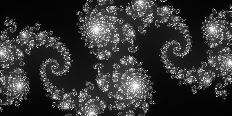
After running the jmain.jl file from the read-eval-print loop (REPL) (or in VS Code), the output to disk should look like that shown in Figure 2.2:

Figure 2.2 – The Julia set generated by the preceding code
After that light relief, it is time to conclude this chapter by introducing a few additional data structures, and we will begin by considering arrays of more than two dimensions—that is, neither vectors nor matrices.


