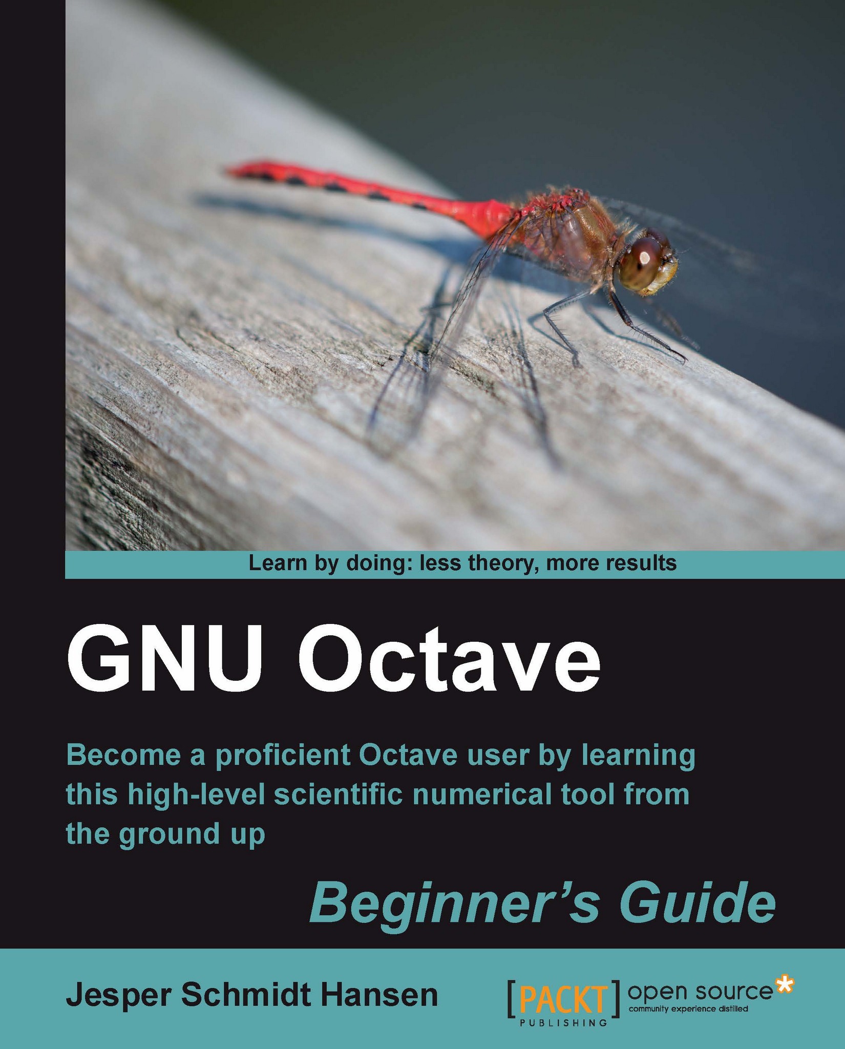
GNU Octave Beginner's Guide: Become a proficient Octave user by learning this high-level scientific numerical tool from the ground up

In the following, we shall see how to instantiate simple variables. By simple variables, we mean scalars, vectors, and matrices. First, a scalar variable with name a is assigned the value 1 by the command:

octave:1> a=1
a = 1

That is, you write the variable name, in this case a, and then you assign a value to the variable using the equal sign. Note that in Octave, variables are not instantiated with a type specifier as it is known from C and other lower-level languages. Octave interprets a number as a real number unless you explicitly tell it otherwise1.

You can display the value of a variable simply by typing the variable name:

octave:2>a
a = 1

Let us move on and instantiate an array of numbers:

octave:3 > b = [1 2 3]
b =
1 2 3

Octave interprets this as the row vector:

(2.1)

rather than a simple one-dimensional array. The elements (or the entries) in a row vector can also be separated by commas, so the command above could have been:

octave:3> b = [1,...

In many real life applications, we have to work with objects that are described by many different types of variables. For example, if we wish to describe the motion of a projectile, it would be useful to know its mass (a scalar), current velocity (a vector), type (a string), and so forth. In Octave, you can instantiate a single variable that contains all this information. These types of variables are named structures and cell arrays.

Structures

A structure in Octave is like a structure in C—it has a name, for example projectile, and contains a set of fields3 that each has a name, as shown in the following figure:

We can refer to the individual structure field using the.character:

structurename.fieldname

where structurename is the name of the structure variable, and fieldname is (as you may have guessed) the field's name.

3or members in C terminology

To show an example of a structure, we can use the projectile described above. Let us therefore name the structure variable...

octave:32>projectile.mass = 10.1
projectile =
{
mass = 10.100
}

octave:33>projectile.velocity = [1 0 0]
projectile =
{
mass = 10.100
velocity =
0 0
}

octave:34>projectile.type = "Cannonball"
projectile =
{
mass = 10.100
velocity =
1 0 0
type = Cannonball
}

and so on for position and whatever else could be relevant.

In this section, we will learn how to obtain information about the variables that have been instantiated. This is particularly useful when you have forgotten the names, sizes, or when you have loaded data from files (more on the latter in Chapter 4).

We are working with quite a few variables now. We can list them all with whos:

octave:48>whos
Variables in the current scope:

Total is 81 elements using 648 bytes

Imagine that you wish to generate a sequence of numbers in the interval -2.1 to 0.5 (including -2.1 and 0.5) with an incremental spacing of 0.2. This is rather tedious to do by hand and is very error prone, because it involves typing a lot of digits. Fortunately, Octave provides you with a very convenient way to do this (note that we now assign the variable b a new value):

octave:60> b = [-2.1:0.2:0.5]
b =
Columns 1 through 7
-2.1000 -1.9000 -1.7000 -1.5000 -1.3000 -1.1000 -0.9000
Columns 8 through 14
-0.7000 -0.5000 -0.3000 -0.1000 0.1000 0.3000 0.5000

If we had done this by hand instead, we should have typed in:

octave:61> size(b)
ans =
1 14

14 numbers. You can also use negative increments if the interval starting value is larger than the end value. If you do not provide an incremental value, Octave assumes 1.

An important point is that if we have chosen an increment of, say 0.4, in Command 60, Octave will give us a number sequence starting from ...

Octave offers easy ways to perform different arithmetic operations. This ranges from simple addition and multiplication to very complicated linear algebra. In this section, we will go through the most basic arithmetic operations, such as addition, subtraction, multiplication, and left and right division. In general, we should think of these operations in the framework of linear algebra and not in terms of arithmetic of simple scalars.

Let us try to perform some of the same operations for multiplication as we did for addition:

octave:75> a*a
ans = 4
octave:76> a*b
ans =
2 4 6
octave:77> b*b
error: operator *: nonconformant arguments (op1 is 1x3, op2 is 1x3)
octave:78> b*c
ans = 14

In the previous section, we discussed the basic arithmetic operations. In this section, we will learn how to compare different variables. Octave (like many other programming languages) uses very intuitive operator characters for this. They are:

For Octave's comparison operators, true is equivalent to a non-zero value and false is equivalent to 0. Let us see a few examples—recall the matrix A from Command 93:

octave:108> A(2,1) == 1
ans = 1
octave:109>A(2,1) == 2
ans = 0
octave:110> A(2,1) > 0
ans = 1
octave:111> A(2,1) != 4
ans = 1

Instead of using != for "not equal to", you can use ~=.

You may be familiar...

Instead of using the left division operator to solve a linear equation system, you can do it "by hand". Let us try this using the equation system given by Equation (2.6) with the solution given in Equation (2.9). First we need to calculate the inverse of A (which exists). This is done via the inv function:

octave:120>inverse_A = inv(A)
inverse_A =
0.2500 -0.1250 -1.0000
0.5000 -0.5000 -1.0000
0.0000 -0.2500 -1.0000

We can now simply perform the matrix multiplication A 1y to get the solution:

octave:121>inverse_A*y
ans =
-1.6250
-2.5000
-2.2500

This output is similar to the output from Command 94. Now, when Octave performs the left division operation, it does not first invert A and then multiply that result with y. Octave has many different algorithms it can use for this operation, depending on the specific nature of the matrix. The results from these algorithms are usually more precise and much quicker than performing the individual steps. In this particular example, it...

We went through a lot of the basics in this chapter! Specifically, we learned:

In the next chapter, we will learn about Octave functions and how to do plotting. We shall make use of many of the things that we have just learned in this chapter.