Shiny can be installed using standard package management functions, as described previously (using the GUI or running install.packages("shiny") at the console).
Let's run some of the examples, as shown in the following code:
> library(shiny)
> runExample("01_hello")
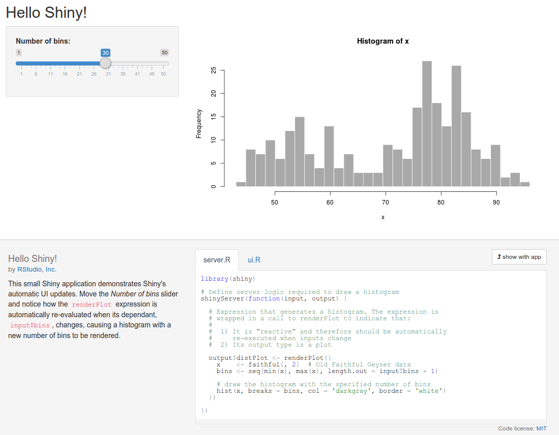
Your web browser should launch and display the following screenshot (note that I clicked on the show below button on the app to better fit the graphic on the page):

The graph shows the frequency of a set of random numbers drawn from a statistical distribution known as the normal distribution, and the slider allows users to select the size of the draw, from 0 to 1,000. You will note that when you move the slider, the graph updates automatically. This is a fundamental feature of Shiny, which makes use of a reactive programming paradigm.
This is a type of programming that uses reactive expressions, which keep track of the values on which they are based. These values can change (they are known as reactive values) and update themselves whenever any of their reactive values change. So, in this example, the function that generates the random data and draws the graph is a reactive expression, and the number of random draws that it makes is a reactive value on which the expression depends. So, whenever the number of draws changes, the function re-executes.
Also, note the layout and style of the web page. Shiny is based by default on the Bootstrap theme (see getbootstrap.com/). However, you are not limited by the styling at all, and can build the whole UI using a mix of HTML, CSS, and Shiny code.
Let's look at an interface that is made with bare-bones HTML and Shiny. Note that in this and all subsequent examples, we're going to assume that you run library(shiny) at the beginning of each session. You don't have to run it before each example, except at the beginning of each R session. So, if you have closed R and have come back, then run it on the console. If you can't remember, run it again to be sure, as follows:
library(shiny)
runExample("08_html")
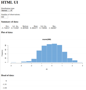
And here it is, in all its customizable glory:

Now, there are a few different statistical distributions to pick from and a different method of selecting the number of observations. By now, you should be looking at the web page and imagining all the possibilities there are to produce your own interactive data summaries and style them just how you want, quickly and simply. By the end of the next chapter, you'll have made your own application with the default UI, and by the end of the book, you'll have complete control over the styling and be pondering where else you can go.
There are lots of other examples included with the Shiny library; just type runExample() in the console to be provided with a list.
To see some really powerful and well-featured Shiny applications, take a look at the showcase at shiny.rstudio.com/gallery/.


