
The standard normal distribution
Recall from Chapter 3, Data Visualization, that the normal distribution's probability density function is:
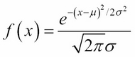
where μ is the population mean and σ is the population standard deviation. Its graph is the well-known bell curve, centered at where x = μ and roughly covering the interval from x = μ–3σ to x = μ+3σ (that is, x = μ±3σ). In theory, the curve is asymptotic to the x axis, never quite touching it, but getting closer as x approaches ±∞.
If a population is normally distributed, then we would expect over 99% of the data points to be within the μ±3σ interval. For example, the American College Board Scholastic Aptitude Test in mathematics (AP math test) was originally set up to have a mean score of μ = 500 and a standard deviation of σ = 100. This would mean that nearly all the scores would fall between μ+3σ = 800 and μ–3σ = 200.
When μ = 0 and σ = 1, we have a special case called the standard normal distribution.

Figure 4-12. The standard normal distribution
Its...