Search icon CANCEL
Subscription
0
Cart icon
Your Cart (0 item)
Close icon
You have no products in your basket yet
Arrow left icon
Explore Products
Best Sellers
New Releases
Books
Videos
Audiobooks
Learning Hub
Free Learning
Arrow right icon
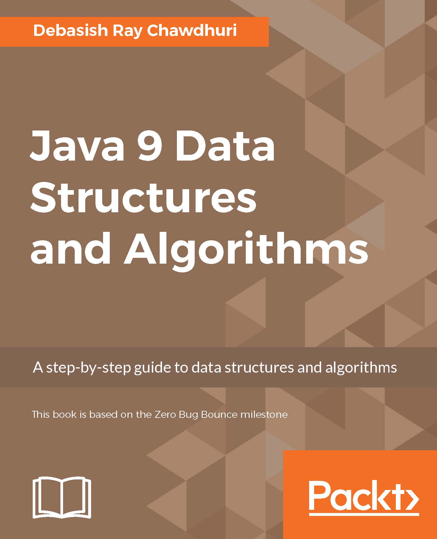
Java 9 Data Structures and Algorithms

Java 9 Data Structures and Algorithms: A step-by-step guide to data structures and algorithms

eBook
€8.99 €26.99
Paperback
€32.99
Subscription
Free Trial
Renews at €18.99p/m

What do you get with Print?

Product feature icon Instant access to your digital eBook copy whilst your Print order is Shipped
Product feature icon Paperback book shipped to your preferred address
Product feature icon Download this book in EPUB and PDF formats
Product feature icon Access this title in our online reader with advanced features
Product feature icon DRM FREE - Read whenever, wherever and however you want
OR
Modal Close icon
Payment Processing...
tick Completed

Shipping Address

Billing Address

Shipping Methods
Table of content icon View table of contents Preview book icon Preview Book

Java 9 Data Structures and Algorithms

Chapter 1. Why Bother? – Basic

Since you already know Java, you have of course written a few programs, which means you have written algorithms. "Well then, what is it?" you might ask. An algorithm is a list of well-defined steps that can be followed by a processor mechanically, or without involving any sort of intelligence, which would produce a desired output in a finite amount of time. Well, that's a long sentence. In simpler words, an algorithm is just an unambiguous list of steps to get something done. It kind of sounds like we are talking about a program. Isn't a program also a list of instructions that we give the computer to follow, in order to get a desired result? Yes it is, and that means an algorithm is really just a program. Well not really, but almost. An algorithm is a program without the details of the particular programming language that we are coding it in. It is the basic idea of the program; think of it as an abstraction of a program where you don't need to bother about the program's syntactic details.

Well, since we already know about programming, and an algorithm is just a program, we are done with it, right? Not really. There is a lot to learn about programs and algorithms, that is, how to write an algorithm to achieve a particular goal. There are, of course, in general, many ways to solve a particular problem and not all ways may be equal. One way may be faster than another, and that is a very important thing about algorithms. When we study algorithms, the time it takes to execute is of utmost importance. In fact, it is the second most important thing about them, the first one being their correctness.

In this chapter, we will take a deeper look into the following ideas:

  • Measuring the performance of an algorithm
  • Asymptotic complexity
  • Why asymptotic complexity matters
  • Why an explicit study of algorithms is important

The performance of an algorithm

No one wants to wait forever to get something done. Making a program run faster surely is important, but how do we know whether a program runs fast? The first logical step would be to measure how many seconds the program takes to run. Suppose we have a program that, given three numbers, a, b, and c, determines the remainder when a raised to the power b is divided by c.

For example, say a=2, b=10, and c = 7, a raised to the power b = 210 = 1024, 1024 % 7 = 2. So, given these values, the program needs to output 2. The following code snippet shows a simple and obvious way of achieving this:

public static long computeRemainder(long base, long power, long divisor){ 
  long baseRaisedToPower = 1;
  for(long i=1;i<=power;i++){ 
    baseRaisedToPower *= base;
  }
  return baseRaisedToPower % divisor;
}

We can now estimate the time it takes by running the program a billion times and checking how long it took to run it, as shown in the following code:

public static void main(String [] args){
  long startTime = System.currentTimeMillis();
  for(int i=0;i<1_000_000_000;i++){
    computeRemainder(2, 10, 7);
  }
  long endTime = System.currentTimeMillis();
  System.out.println(endTime - startTime);
}

On my computer, it takes 4,393 milliseconds. So the time taken per call is 4,393 divided by a billion, that is, about 4.4 nanoseconds. Looks like a very reasonable time to do any computation. But what happens if the input is different? What if I pass power = 1000? Let's check that out. Now it takes about 420,000 milliseconds to run a billion times, or about 420 nanoseconds per run. Clearly, the time taken to do this computation depends on the input, and that means any reasonable way to talk about the performance of a program needs to take into account the input to the program.

Okay, so we can say that the number of nanoseconds our program takes to run is 0.42 X power, approximately.

If you run the program with the input (2, 1000, and 7), you will get an output of 0, which is not correct. The correct output is 2. So, what is going on here? The answer is that the maximum value that a long type variable can hold is one less than 2 raised to the power 63, or 9223372036854775807L. The value 2 raised to the power 1,000 is, of course, much more than this, causing the value to overflow, which brings us to our next point: how much space does a program need in order to run?

In general, the memory space required to run a program can be measured in terms of the bytes required for the program to operate. Of course, it requires the space to at least store the input and the output. It may as well need some additional space to run, which is called auxiliary space. It is quite obvious that just like time, the space required to run a program would, in general, also be dependent on the input.

In the case of time, apart from the fact that the time depends on the input, it also depends on which computer you are running it on. The program that takes 4 seconds to run on my computer may take 40 seconds on a very old computer from the nineties and may run in 2 seconds in yours. However, the actual computer you run it on only improves the time by a constant multiplier. To avoid getting into too much detail about specifying the details of the hardware the program is running on, instead of saying the program takes 0.42 X power milliseconds approximately, we can say the time taken is a constant times the power, or simply say it is proportional to the power.

Saying the computation time is proportional to the power actually makes it so non-specific to hardware, or even the language the program is written in, that we can estimate this relationship by just looking at the program and analyzing it. Of course, the running time is sort of proportional to the power because there is a loop that executes power number of times, except, of course, when the power is so small that the other one-time operations outside the loop actually start to matter.

Best case, worst case and the average case complexity

In general, the time or space required for an algorithm to process a certain input depends not only on the size of the input, but also on the actual value of the input. For example, a certain algorithm to arrange a list of values in increasing order may take much less time if the input is already sorted than when it is an arbitrary unordered list. This is why, in general, we must have a different function representing the time or space required in the different cases of input. However, the best case scenario would be where the resources required for a certain size of an input take the least amount of resources. The would also be a worst case scenario, in which the algorithm needs the maximum amount of resources for a certain size of input. An average case is an estimation of the resources taken for a given size of inputs averaged over all values of the input with that size weighted by their probability of occurrence.

Analysis of asymptotic complexity

We seem to have hit upon an idea, an abstract sense of the running time. Let's spell it out. In an abstract way, we analyze the running time of and the space required by a program by using what is known as the asymptotic complexity.

We are only interested in what happens when the input is very large because it really does not matter how long it takes for a small input to be processed; it's going to be small anyway. So, if we have x3 + x2, and if x is very large, it's almost the same as x3. We also don't want to consider constant factors of a function, as we have pointed out earlier, because it is dependent on the particular hardware we are running the program on and the particular language we have implemented it in. An algorithm implemented in Java will perform a constant times slower than the same algorithm written in C. The formal way of tackling these abstractions in defining the complexity of an algorithm is called an asymptotic bound. Strictly speaking, an asymptotic bound is for a function and not for an algorithm. The idea is to first express the time or space required for a given algorithm to process an input as a function of the size of the input in bits and then looking for an asymptotic bound of that function.

We will consider three types of asymptotic bounds—an upper bound, a lower bound and a tight bound. We will discuss these in the following sections.

Asymptotic upper bound of a function

An upper bound, as the name suggests, puts an upper limit of a function's growth. The upper bound is another function that grows at least as fast as the original function. What is the point of talking about one function in place of another? The function we use is in general a lot more simplified than the actual function for computing running time or space required to process a certain size of input. It is a lot easier to compare simplified functions than to compare complicated functions.

For a function f, we define the notation O, called big O, in the following ways:

  1. f(x) = O(f(x)).
    • For example, x3 = O(x3).
  2. If f(x) = O(g(x)), then k f(x) = O(g(x)) for any non-zero constant k.
    • For example, 5x3 = O(x3) and 2 log x = O(log x) and -x3 = O(x3) (taking k= -1).
  3. If f(x) = O(g(x)) and |h(x)|<|f(x)| for all sufficiently large x, then f(x) + h(x) = O(g(x)).
    • For example, 5x3 - 25x2 + 1 = O(x3) because for a sufficiently large x, |- 25x2 + 1| = 25x2 - 1 is much less that | 5x3| = 5x3. So, f(x) + g(x) = 5x3 - 25x2 + 1 = O(x3) as f(x) = 5x3 = O(x3).
    • We can prove by similar logic that x3 = O( 5x3 - 25x2 + 1).
  4. if f(x) = O(g(x)) and |h(x)| > |g(x)| for all sufficiently large x, then f(x) = O(h(x)).
    • For example, x3 = O(x4), because if x is sufficiently large, x4 > x3.

Note that whenever there is an inequality on functions, we are only interested in what happens when x is large; we don't bother about what happens for small x.

Note

To summarize the above definition, you can drop constant multipliers (rule 2) and ignore lower order terms (rule 3). You can also overestimate (rule 4). You can also do all combinations for those because rules can be applied any number of times.

We had to consider the absolute values of the function to cater to the case when values are negative, which never happens in running time, but we still have it for completeness.

Note

There is something about the sign = that is not usual. Just because f(x) = O(g(x)), it does not mean, O(g(x)) = f(x). In fact, the last one does not even mean anything.

It is enough for all purposes to just know the preceding definition of the big O notation. You can read the following formal definition if you are interested. Otherwise you can skip the rest of this subsection.

The preceding idea can be summarized in a formal way. We say the expression f(x) = O(g(x)) means that positive constants M and x0 exist, such that |f(x)| < M|g(x)| whenever x > x0. Remember that you just have to find one example of M and x0 that satisfy the condition, to make the assertion f(x) = O(g(x)).

For example, Figure 1 shows an example of a function T(x) = 100x2 +2000x+200. This function is O(x2 ), with some x0 = 11 and M = 300. The graph of 300x2 overcomes the graph of T(x) at x=11 and then stays above T(x) up to infinity. Notice that the function 300x2 is lower than T(x) for smaller values of x, but that does not affect our conclusion.

Asymptotic upper bound of a function

Figure 1. Asymptotic upper bound

To see that it's the same thing as the previous four points, first think of x0 as the way to ensure that x is sufficiently large. I leave it up to you to prove the above four conditions from the formal definition.

I will, however, show some examples of using the formal definition:

  • 5x2 = O(x2) because we can say, for example, x0 = 10 and M = 10 and thus f(x) < Mg(x) whenever x > x0, that is, 5x2 < 10x2 whenever x > 10.
  • It is also true that 5x2 = O(x3) because we can say, for example, x0 = 10 and M = 10 and thus f(x) < Mg(x) whenever x > x0, that is, 5x2 < 10x3 whenever x > 10. This highlights a point that if f(x) = O(g(x)), it is also true that f(x) = O(h(x)) if h(x) is some functions that grows at least as fast as f(x).
  • How about the function f(x) = 5x2 - 10x + 3? We can easily see that when x is sufficiently large, 5x2 will far surpass the term 10x. To prove my point, I can simply say x>5, 5x2> 10x. Every time we increment x by one, the increment in 5x2 is 10x + 1 and the increment in 10x is just a constant, 10. 10x+1 > 10 for all positive x, so it is easy to see why 5x2 is always going to stay above 10x as x goes higher and higher.

In general, any polynomial of the form an xn + an-1 xn-1 + an-2 xn-2 + … + a0 = O(xn). To show this, we will first see that a0 = O(1). This is true because we can have x0 = 1 and M = 2|a0|, and we will have |a0| < 2|a0 | whenever x > 1.

Now, let us assume it is true for some n. Thus, an xn + an-1 xn-1 + an-2 xn-2 + … + a0 = O(xn). What it means, of course, is that some Mn and x0 exist, such that |an xn + an-1 xn-1 + an-2 xn-2 + … + a0 | < Mn xn whenever x>x0. We can safely assume that x0 >2, because if it is not so, we can simply add 2 to it to get a new x0, which is at least 2.

Now, |an xn + an-1 xn-1 + an-2 xn-2 + … + a0 | < Mn xn implies |an+1 xn+1 + an xn + an-1 xn-1 + an-2 xn-2 + … + a0 | ≤ |an+1 xn+1 | + |anxn + an-1 xn-1 + an-2 xn-2 + … + a0 | < |an+1 xn+1 | + Mn xn.

This means |an+1 xn+1 | + Mn xn > |an xn + an-1 xn-1 + an-2 xn-2 + … + a0 |.

If we take Mn+1 = |an+1 | + Mn, we can see that Mn+1 xn+1 = |an+1 | xn+1 + Mn xn+1 =|an+1 xn+1 | + Mn xn+1 > |an+1 xn+1 | + Mn xn > |an+1 xn+1 + an xn + an-1 xn-1 + an-2 xn-2 + … + a0 |.

That is to say, |an+1 xn+1 + an-1 xn-1 + an-2 xn-2 + … + a0 |< Mn+1 xn+1 for all x > x0, that is, an+1 xn+1 + an xn + an-1 xn-1 + an-2 xn-2 + … + a0 = O(xn+1 ).

Now, we have it true for n=0, that is, a0 = O(1). This means, by our last conclusion, a 1x + a0 = O(x). This means, by the same logic, a2 x2 + a1 x + a0 = O(x2 ), and so on. We can easily see that this means it is true for all polynomials of positive integral degrees.

Asymptotic upper bound of an algorithm

Okay, so we figured out a way to sort of abstractly specify an upper bound on a function that has one argument. When we talk about the running time of a program, this argument has to contain information about the input. For example, in our algorithm, we can say, the execution time equals O(power). This scheme of specifying the input directly will work perfectly fine for all programs or algorithms solving the same problem because the input will be the same for all of them. However, we might want to use the same technique to measure the complexity of the problem itself: it is the complexity of the most efficient program or algorithm that can solve the problem. If we try to compare the complexity of different problems, though, we will hit a wall because different problems will have different inputs. We must specify the running time in terms of something that is common among all problems, and that something is the size of the input in bits or bytes. How many bits do we need to express the argument, power, when it's sufficiently large? Approximately log2 (power). So, in specifying the running time, our function needs to have an input that is of the size log2 (power) or lg (power). We have seen that the running time of our algorithm is proportional to the power, that is, constant times power, which is constant times 2 lg(power) = O(2x),where x= lg(power), which is the the size of the input.

Asymptotic lower bound of a function

Sometimes, we don't want to praise an algorithm, we want to shun it; for example, when the algorithm is written by someone we don't like or when some algorithm is really poorly performing. When we want to shun it for its horrible performance, we may want to talk about how badly it performs even for the best input. An a symptotic lower bound can be defined just like how greater-than-or-equal-to can be defined in terms of less-than-or-equal-to.

A function f(x) = Ω(g(x)) if and only if g(x) = O(f(x)). The following list shows a few examples:

  • Since x3 = O(x3), x3 = Ω(x3)
  • Since x3 = O(5x3), 5x3 = Ω(x3)
  • Since x3 = O(5x3 - 25x2 + 1), 5x3 - 25x2 + 1 = Ω(x3)
  • Since x3 = O(x4), x4 = O(x3)

Again, for those of you who are interested, we say the expression f(x) = Ω(g(x)) means there exist positive constants M and x0, such that |f(x)| > M|g(x)| whenever x > x0, which is the same as saying |g(x)| < (1/M)|f(x)| whenever x > x0, that is, g(x) = O(f(x)).

The preceding definition was introduced by Donald Knuth, which was a stronger and more practical definition to be used in computer science. Earlier, there was a different definition of the lower bound Ω that is more complicated to understand and covers a few more edge cases. We will not talk about edge cases here.

While talking about how horrible an algorithm is, we can use an asymptotic lower bound of the best case to really make our point. However, even a criticism of the worst case of an algorithm is quite a valid argument. We can use an asymptotic lower bound of the worst case too for this purpose, when we don't want to find out an asymptotic tight bound. In general, the asymptotic lower bound can be used to show a minimum rate of growth of a function when the input is large enough in size.

Asymptotic tight bound of a function

There is another kind of bound that sort of means equality in terms of asymptotic complexity. A theta bound is specified as f(x) = Ͽ(g(x)) if and only if f(x) = O(g(x)) and f(x) = Ω(g(x)). Let's see some examples to understand this even better:

  • Since 5x3=O(x3) and also 5x3=Ω(x3), we have 5x3=Ͽ(x3)
  • Since 5x3 + 4x2=O(x3) and 5x3 + 4x2=Ω(x3), we have 5x3 + 4x2=O(x3)
  • However, even though 5x3 + 4x2 =O(x4), since it is not Ω(x4), it is also not Ͽ(x4)
  • Similarly, 5x3 + 4x2 is not Ͽ(x2) because it is not O(x2)

In short, you can ignore constant multipliers and lower order terms while determining the tight bound, but you cannot choose a function which grows either faster or slower than the given function. The best way to check whether the bound is right is to check the O and the condition separately, and say it has a theta bound only if they are the same.

Note that since the complexity of an algorithm depends on the particular input, in general, the tight bound is used when the complexity remains unchanged by the nature of the input.

In some cases, we try to find the average case complexity, especially when the upper bound really happens only in the case of an extremely pathological input. But since the average must be taken in accordance with the probability distribution of the input, it is not just dependent on the algorithm itself. The bounds themselves are just bounds for particular functions and not for algorithms. However, the total running time of an algorithm can be expressed as a grand function that changes it's formula as per the input, and that function may have different upper and lower bounds. There is no sense in talking about an asymptotic average bound because, as we discussed, the average case is not just dependent on the algorithm itself, but also on the probability distribution of the input. The average case is thus stated as a function that would be a probabilistic average running time for all inputs, and, in general, the asymptotic upper bound of that average function is reported.

Optimization of our algorithm

Before we dive into actually optimizing algorithms, we need to first correct our algorithm for large powers. We will use some tricks to do so, as described below.

Fixing the problem with large powers

Equipped with all the toolboxes of asymptotic analysis, we will start optimizing our algorithm. However, since we have already seen that our program does not work properly for even moderately large values of power, let's first fix that. There are two ways of fixing this; one is to actually give the amount of space it requires to store all the intermediate products, and the other is to do a trick to limit all the intermediate steps to be within the range of values that the long datatype can support. We will use binomial theorem to do this part.

As a reminder, binomial theorem says (x+y)n = xn + n C1 xn-1 y + n C2 xn-2 y2 + n C3 xn-3 y3 + n C4 xn-4 y4 + … n Cn-1 x1 yn-1 + yn for positive integral values of n. The important point here is that all the coefficients are integers. Suppose, r is the remainder when we divide a by b. This makes a = kb + r true for some positive integer k. This means r = a-kb, and rn = (a-kb)n.

If we expand this using binomial theorem, we have rn = an - n C1 an-1 .kb + n C2 an-2 .(kb)2 - n C3 an-3 .(kb)3 + n C4 an-4 .(kb)4 + … n Cn-1 a1 .(kb)n-1 ± (kb)n.

Note that apart from the first term, all other terms have b as a factor. Which means that we can write rn = an + bM for some integer M. If we divide both sides by b now and take the remainder, we have rn % b = an % b, where % is the Java operator for finding the remainder.

The idea now would be to take the remainder by the divisor every time we raise the power. This way, we will never have to store more than the range of the remainder:

public static long computeRemainderCorrected(long base, long power, long divisor){
  long baseRaisedToPower = 1;
  for(long i=1;i<=power;i++){
    baseRaisedToPower *= base;
    baseRaisedToPower %= divisor;
  }
  return baseRaisedToPower;
}

This program obviously does not change the time complexity of the program; it just fixes the problem with large powers. The program also maintains a constant space complexity.

Improving time complexity

The current running time complexity is O(2x ), where x is the size of the input as we have already computed. Can we do better than this? Let's see.

What we need to compute is (basepower ) % divisor. This is, of course, the same as (base2)power/2 % divisor. If we have an even power, we have reduced the number of operations by half. If we can keep doing this, we can raise the power of base by 2n in just n steps, which means our loop only has to run lg(power) times, and hence, the complexity is O(lg(2x )) = O(x), where x is the number of bits to store power. This is a substantial reduction in the number of steps to compute the value for large powers.

However, there is a catch. What happens if the power is not divisible by 2? Well, then we can write (basepower )% divisor = (base ((basepower-1 ))%divisor = (base ((base2)power-1 )%divisor, and power-1 is, of course, even and the computation can proceed. We will write up this code in a program. The idea is to start from the most significant bit and move towards less and less significant bits. If a bit with 1 has n bits after it, it represents multiplying the result by the base and then squaring n times after this bit. We accumulate this squaring by squaring for the subsequent steps. If we find a zero, we keep squaring for the sake of accumulating squaring for the earlier bits:

public static long computeRemainderUsingEBS(long base, long power, long divisor){
  long baseRaisedToPower = 1;
  long powerBitsReversed = 0;
  int numBits=0;

First reverse the bits of our power so that it is easier to access them from the least important side, which is more easily accessible. We also count the number of bits for later use:

  while(power>0){
    powerBitsReversed <<= 1;
    powerBitsReversed += power & 1;
    power >>>= 1;
    numBits++;
  }

Now we extract one bit at a time. Since we have already reversed the order of bit, the first one we get is the most significant one. Just to get an intuition on the order, the first bit we collect will eventually be squared the maximum number of times and hence will act like the most significant bit:

  while (numBits-->0){
    if(powerBitsReversed%2==1){
      baseRaisedToPower *= baseRaisedToPower * base;
    }else{
      baseRaisedToPower *= baseRaisedToPower;
    }
    baseRaisedToPower %= divisor;
    powerBitsReversed>>>=1;
  }
  return baseRaisedToPower;
}

We test the performance of the algorithm; we compare the time taken for the same computation with the earlier and final algorithms with the following code:

public static void main(String [] args){
  System.out.println(computeRemainderUsingEBS(13, 10_000_000, 7));

  long startTime = System.currentTimeMillis();
  for(int i=0;i<1000;i++){
    computeRemainderCorrected(13, 10_000_000, 7);
  } 
  long endTime = System.currentTimeMillis();
  System.out.println(endTime - startTime);

  startTime = System.currentTimeMillis();
  for(int i=0;i<1000;i++){
    computeRemainderUsingEBS(13, 10_000_000, 7);
  }
  endTime = System.currentTimeMillis();
  System.out.println(endTime - startTime);
}

The first algorithm takes 130,190 milliseconds to complete all 1,000 times execution on my computer and the second one takes just 2 milliseconds to do the same. This clearly shows the tremendous gain in performance for a large power like 10 million. The algorithm for squaring the term repeatedly to achieve exponentiation like we did is called... well, exponentiation by squaring. This example should be able to motivate you to study algorithms for the sheer obvious advantage it can give in improving the performance of computer programs.

Summary

In this chapter, you saw how we can think about measuring the running time of and the memory required by an algorithm in seconds and bytes, respectively. Since this depends on the particular implementation, the programming platform, and the hardware, we need a notion of talking about running time in an abstract way. Asymptotic complexity is a measure of the growth of a function when the input is very large. We can use it to abstract our discussion on running time. This is not to say that a programmer should not spend any time to make a run a program twice as fast, but that comes only after the program is already running at the minimum asymptotic complexity.

We also saw that the asymptotic complexity is not just a property of the problem at hand that we are trying to solve, but also a property of the particular way we are solving it, that is, the particular algorithm we are using. We also saw that two programs solving the same problem while running different algorithms with different asymptotic complexities can perform vastly differently for large inputs. This should be enough motivation to study algorithms explicitly.

In the following chapters, we will study the most used algorithmic tricks and concepts required in daily use. We will start from the very easy ones that are also the building blocks for the more advanced techniques. This book is, of course, by no means comprehensive; the objective is to provide enough background to make you comfortable with the basic concepts and then you can read on.

Left arrow icon Right arrow icon
Download code icon Download Code

Key benefits

  • This book provides complete coverage of reactive and functional data structures
  • Based on the latest version of Java 9, this book illustrates the impact of new features on data structures
  • Gain exposure to important concepts such as Big-O Notation and Dynamic Programming

Description

Java 9 Data Structures and Algorithms covers classical, functional, and reactive data structures, giving you the ability to understand computational complexity, solve problems, and write efficient code. This book is based on the Zero Bug Bounce milestone of Java 9. We start off with the basics of algorithms and data structures, helping you understand the fundamentals and measure complexity. From here, we introduce you to concepts such as arrays, linked lists, as well as abstract data types such as stacks and queues. Next, we’ll take you through the basics of functional programming while making sure you get used to thinking recursively. We provide plenty of examples along the way to help you understand each concept. You will also get a clear picture of reactive programming, binary searches, sorting, search trees, undirected graphs, and a whole lot more!

Who is this book for?

This book is for Java developers who want to learn about data structures and algorithms. Basic knowledge of Java is assumed.

What you will learn

  • Understand the fundamentals of algorithms, data structures, and measurement of complexity
  • Find out what general purpose data structures are, including arrays, linked lists, double ended linked lists, and circular lists
  • Get a grasp on the basics of abstract data types—stack, queue, and double ended queue
  • See how to use recursive functions and immutability while understanding and in terms of recursion
  • Handle reactive programming and its related data structures
  • Use binary search, sorting, and efficient sorting—quicksort and merge sort
  • Work with the important concept of trees and list all nodes of the tree, traversal of tree, search trees, and balanced search trees
  • Apply advanced general purpose data structures, priority queue-based sorting, and random access immutable linked lists
  • Gain a better understanding of the concept of graphs, directed and undirected graphs, undirected trees, and much more
Estimated delivery fee Deliver to Sweden

Premium delivery 7 - 10 business days

€17.95
(Includes tracking information)

Product Details

Country selected
Publication date, Length, Edition, Language, ISBN-13
Publication date : Apr 28, 2017
Length: 340 pages
Edition : 1st
Language : English
ISBN-13 : 9781785889349
Vendor :
Oracle
Category :
Languages :

What do you get with Print?

Product feature icon Instant access to your digital eBook copy whilst your Print order is Shipped
Product feature icon Paperback book shipped to your preferred address
Product feature icon Download this book in EPUB and PDF formats
Product feature icon Access this title in our online reader with advanced features
Product feature icon DRM FREE - Read whenever, wherever and however you want
OR
Modal Close icon
Payment Processing...
tick Completed

Shipping Address

Billing Address

Shipping Methods
Estimated delivery fee Deliver to Sweden

Premium delivery 7 - 10 business days

€17.95
(Includes tracking information)

Product Details

Publication date : Apr 28, 2017
Length: 340 pages
Edition : 1st
Language : English
ISBN-13 : 9781785889349
Vendor :
Oracle
Category :
Languages :

Packt Subscriptions

See our plans and pricing
Modal Close icon
€18.99 billed monthly
Feature tick icon Unlimited access to Packt's library of 7,000+ practical books and videos
Feature tick icon Constantly refreshed with 50+ new titles a month
Feature tick icon Exclusive Early access to books as they're written
Feature tick icon Solve problems while you work with advanced search and reference features
Feature tick icon Offline reading on the mobile app
Feature tick icon Simple pricing, no contract
€189.99 billed annually
Feature tick icon Unlimited access to Packt's library of 7,000+ practical books and videos
Feature tick icon Constantly refreshed with 50+ new titles a month
Feature tick icon Exclusive Early access to books as they're written
Feature tick icon Solve problems while you work with advanced search and reference features
Feature tick icon Offline reading on the mobile app
Feature tick icon Choose a DRM-free eBook or Video every month to keep
Feature tick icon PLUS own as many other DRM-free eBooks or Videos as you like for just €5 each
Feature tick icon Exclusive print discounts
€264.99 billed in 18 months
Feature tick icon Unlimited access to Packt's library of 7,000+ practical books and videos
Feature tick icon Constantly refreshed with 50+ new titles a month
Feature tick icon Exclusive Early access to books as they're written
Feature tick icon Solve problems while you work with advanced search and reference features
Feature tick icon Offline reading on the mobile app
Feature tick icon Choose a DRM-free eBook or Video every month to keep
Feature tick icon PLUS own as many other DRM-free eBooks or Videos as you like for just €5 each
Feature tick icon Exclusive print discounts

Frequently bought together


Stars icon
Total 111.97
Java 9 Concurrency Cookbook, Second Edition
€41.99
Java 9 Data Structures and Algorithms
€32.99
Java 9 Programming By Example
€36.99
Total 111.97 Stars icon
Banner background image

Table of Contents

12 Chapters
1. Why Bother? – Basic Chevron down icon Chevron up icon
2. Cogs and Pulleys – Building Blocks Chevron down icon Chevron up icon
3. Protocols – Abstract Data Types Chevron down icon Chevron up icon
4. Detour – Functional Programming Chevron down icon Chevron up icon
5. Efficient Searching – Binary Search and Sorting Chevron down icon Chevron up icon
6. Efficient Sorting – quicksort and mergesort Chevron down icon Chevron up icon
7. Concepts of Tree Chevron down icon Chevron up icon
8. More About Search – Search Trees and Hash Tables Chevron down icon Chevron up icon
9. Advanced General Purpose Data Structures Chevron down icon Chevron up icon
10. Concepts of Graph Chevron down icon Chevron up icon
11. Reactive Programming Chevron down icon Chevron up icon
Index Chevron down icon Chevron up icon

Customer reviews

Rating distribution
Full star icon Full star icon Half star icon Empty star icon Empty star icon 2.3
(3 Ratings)
5 star 0%
4 star 33.3%
3 star 0%
2 star 33.3%
1 star 33.3%
madhu Feb 01, 2022
Full star icon Full star icon Full star icon Full star icon Empty star icon 4
I like this book .
Amazon Verified review Amazon
Bin Jul 24, 2018
Full star icon Full star icon Empty star icon Empty star icon Empty star icon 2
This book is confusing. I do not recommend.
Amazon Verified review Amazon
RAGHVENDRA KUMAR Feb 25, 2018
Full star icon Empty star icon Empty star icon Empty star icon Empty star icon 1
i want to return this book very pages is very poor condition
Amazon Verified review Amazon
Get free access to Packt library with over 7500+ books and video courses for 7 days!
Start Free Trial

FAQs

What is the delivery time and cost of print book? Chevron down icon Chevron up icon

Shipping Details

USA:

'

Economy: Delivery to most addresses in the US within 10-15 business days

Premium: Trackable Delivery to most addresses in the US within 3-8 business days

UK:

Economy: Delivery to most addresses in the U.K. within 7-9 business days.
Shipments are not trackable

Premium: Trackable delivery to most addresses in the U.K. within 3-4 business days!
Add one extra business day for deliveries to Northern Ireland and Scottish Highlands and islands

EU:

Premium: Trackable delivery to most EU destinations within 4-9 business days.

Australia:

Economy: Can deliver to P. O. Boxes and private residences.
Trackable service with delivery to addresses in Australia only.
Delivery time ranges from 7-9 business days for VIC and 8-10 business days for Interstate metro
Delivery time is up to 15 business days for remote areas of WA, NT & QLD.

Premium: Delivery to addresses in Australia only
Trackable delivery to most P. O. Boxes and private residences in Australia within 4-5 days based on the distance to a destination following dispatch.

India:

Premium: Delivery to most Indian addresses within 5-6 business days

Rest of the World:

Premium: Countries in the American continent: Trackable delivery to most countries within 4-7 business days

Asia:

Premium: Delivery to most Asian addresses within 5-9 business days

Disclaimer:
All orders received before 5 PM U.K time would start printing from the next business day. So the estimated delivery times start from the next day as well. Orders received after 5 PM U.K time (in our internal systems) on a business day or anytime on the weekend will begin printing the second to next business day. For example, an order placed at 11 AM today will begin printing tomorrow, whereas an order placed at 9 PM tonight will begin printing the day after tomorrow.


Unfortunately, due to several restrictions, we are unable to ship to the following countries:

  1. Afghanistan
  2. American Samoa
  3. Belarus
  4. Brunei Darussalam
  5. Central African Republic
  6. The Democratic Republic of Congo
  7. Eritrea
  8. Guinea-bissau
  9. Iran
  10. Lebanon
  11. Libiya Arab Jamahriya
  12. Somalia
  13. Sudan
  14. Russian Federation
  15. Syrian Arab Republic
  16. Ukraine
  17. Venezuela
What is custom duty/charge? Chevron down icon Chevron up icon

Customs duty are charges levied on goods when they cross international borders. It is a tax that is imposed on imported goods. These duties are charged by special authorities and bodies created by local governments and are meant to protect local industries, economies, and businesses.

Do I have to pay customs charges for the print book order? Chevron down icon Chevron up icon

The orders shipped to the countries that are listed under EU27 will not bear custom charges. They are paid by Packt as part of the order.

List of EU27 countries: www.gov.uk/eu-eea:

A custom duty or localized taxes may be applicable on the shipment and would be charged by the recipient country outside of the EU27 which should be paid by the customer and these duties are not included in the shipping charges been charged on the order.

How do I know my custom duty charges? Chevron down icon Chevron up icon

The amount of duty payable varies greatly depending on the imported goods, the country of origin and several other factors like the total invoice amount or dimensions like weight, and other such criteria applicable in your country.

For example:

  • If you live in Mexico, and the declared value of your ordered items is over $ 50, for you to receive a package, you will have to pay additional import tax of 19% which will be $ 9.50 to the courier service.
  • Whereas if you live in Turkey, and the declared value of your ordered items is over € 22, for you to receive a package, you will have to pay additional import tax of 18% which will be € 3.96 to the courier service.
How can I cancel my order? Chevron down icon Chevron up icon

Cancellation Policy for Published Printed Books:

You can cancel any order within 1 hour of placing the order. Simply contact customercare@packt.com with your order details or payment transaction id. If your order has already started the shipment process, we will do our best to stop it. However, if it is already on the way to you then when you receive it, you can contact us at customercare@packt.com using the returns and refund process.

Please understand that Packt Publishing cannot provide refunds or cancel any order except for the cases described in our Return Policy (i.e. Packt Publishing agrees to replace your printed book because it arrives damaged or material defect in book), Packt Publishing will not accept returns.

What is your returns and refunds policy? Chevron down icon Chevron up icon

Return Policy:

We want you to be happy with your purchase from Packtpub.com. We will not hassle you with returning print books to us. If the print book you receive from us is incorrect, damaged, doesn't work or is unacceptably late, please contact Customer Relations Team on customercare@packt.com with the order number and issue details as explained below:

  1. If you ordered (eBook, Video or Print Book) incorrectly or accidentally, please contact Customer Relations Team on customercare@packt.com within one hour of placing the order and we will replace/refund you the item cost.
  2. Sadly, if your eBook or Video file is faulty or a fault occurs during the eBook or Video being made available to you, i.e. during download then you should contact Customer Relations Team within 14 days of purchase on customercare@packt.com who will be able to resolve this issue for you.
  3. You will have a choice of replacement or refund of the problem items.(damaged, defective or incorrect)
  4. Once Customer Care Team confirms that you will be refunded, you should receive the refund within 10 to 12 working days.
  5. If you are only requesting a refund of one book from a multiple order, then we will refund you the appropriate single item.
  6. Where the items were shipped under a free shipping offer, there will be no shipping costs to refund.

On the off chance your printed book arrives damaged, with book material defect, contact our Customer Relation Team on customercare@packt.com within 14 days of receipt of the book with appropriate evidence of damage and we will work with you to secure a replacement copy, if necessary. Please note that each printed book you order from us is individually made by Packt's professional book-printing partner which is on a print-on-demand basis.

What tax is charged? Chevron down icon Chevron up icon

Currently, no tax is charged on the purchase of any print book (subject to change based on the laws and regulations). A localized VAT fee is charged only to our European and UK customers on eBooks, Video and subscriptions that they buy. GST is charged to Indian customers for eBooks and video purchases.

What payment methods can I use? Chevron down icon Chevron up icon

You can pay with the following card types:

  1. Visa Debit
  2. Visa Credit
  3. MasterCard
  4. PayPal
What is the delivery time and cost of print books? Chevron down icon Chevron up icon

Shipping Details

USA:

'

Economy: Delivery to most addresses in the US within 10-15 business days

Premium: Trackable Delivery to most addresses in the US within 3-8 business days

UK:

Economy: Delivery to most addresses in the U.K. within 7-9 business days.
Shipments are not trackable

Premium: Trackable delivery to most addresses in the U.K. within 3-4 business days!
Add one extra business day for deliveries to Northern Ireland and Scottish Highlands and islands

EU:

Premium: Trackable delivery to most EU destinations within 4-9 business days.

Australia:

Economy: Can deliver to P. O. Boxes and private residences.
Trackable service with delivery to addresses in Australia only.
Delivery time ranges from 7-9 business days for VIC and 8-10 business days for Interstate metro
Delivery time is up to 15 business days for remote areas of WA, NT & QLD.

Premium: Delivery to addresses in Australia only
Trackable delivery to most P. O. Boxes and private residences in Australia within 4-5 days based on the distance to a destination following dispatch.

India:

Premium: Delivery to most Indian addresses within 5-6 business days

Rest of the World:

Premium: Countries in the American continent: Trackable delivery to most countries within 4-7 business days

Asia:

Premium: Delivery to most Asian addresses within 5-9 business days

Disclaimer:
All orders received before 5 PM U.K time would start printing from the next business day. So the estimated delivery times start from the next day as well. Orders received after 5 PM U.K time (in our internal systems) on a business day or anytime on the weekend will begin printing the second to next business day. For example, an order placed at 11 AM today will begin printing tomorrow, whereas an order placed at 9 PM tonight will begin printing the day after tomorrow.


Unfortunately, due to several restrictions, we are unable to ship to the following countries:

  1. Afghanistan
  2. American Samoa
  3. Belarus
  4. Brunei Darussalam
  5. Central African Republic
  6. The Democratic Republic of Congo
  7. Eritrea
  8. Guinea-bissau
  9. Iran
  10. Lebanon
  11. Libiya Arab Jamahriya
  12. Somalia
  13. Sudan
  14. Russian Federation
  15. Syrian Arab Republic
  16. Ukraine
  17. Venezuela