Asymptotic analysis

When building a service, it's imperative that it finds information quickly, otherwise it could mean the difference between success or failure for your product. There is no single data structure or algorithm that offers optimal performance in all use cases. In order to know which is the best solution, we need to have a way to evaluate how long it takes an algorithm to run. Almost any algorithm is sufficiently efficient when running on a small number of inputs. When we're talking about measuring the cost or complexity of an algorithm, what we're really talking about is performing an analysis of the algorithm when the input sets are very large. Analyzing what happens as the number of inputs approaches infinity is referred to as asymptotic analysis. It allows us to answer questions such as:

• How much space is needed in the worst case?
• How long will an algorithm take to run with a given input size?
• Can the problem be solved?

For example, when analyzing the running time of a function that sorts a list of numbers, we're concerned with how long it takes as a function of the size of the input. As an example, when we compare sorting algorithms, we say the average insertion sort takes time T(n), where T(n) = c*n²+K for some constants c and k, which represents a quadratic running time. Now compare that to merge sort, which takes time T(n), where T(n) = c*n*log₂(n)+k for some constants c and k, which represents a linearithmic running time.

We typically ignore smaller values of x since we're generally interested in estimating how slow an algorithm will be on larger data inputs. The asymptotic behavior of the merge sort function f(x), such that f(x) = c*x*log₂(x)+k, refers to the growth of f(x) as x gets larger.

Generally, the slower the asymptotic growth rate, the better the algorithm, although this is not a hard and fast rule. By this allowance, a linear algorithm, f(x) = d*x+k, is always asymptotically better than a linearithmic algorithm, f(x) = c*x*log₂(x)+q. This is because where c, d, k, and q > 0 there is always some x at which the magnitude of c*x*log₂(x)+q overtakes d*x+k.

Order of growth

In estimating the running time for the preceding sort algorithms, we don't know what the constants c or k are. We know they are a constant of modest size, but other than that, it is not important. From our asymptotic analysis, we know that the log-linear merge sort is faster than the insertion sort, which is quadratic, even though their constants differ. We might not even be able to measure the constants directly because of CPU instruction sets and programming language differences. These estimates are usually only accurate up to a constant factor; for these reasons, we usually ignore constant factors in comparing asymptotic running times.

In computer science, Big-O is the most commonly used asymptotic notation for comparing functions, which also has a convenient notation for hiding the constant factor of an algorithm. Big-O compares functions expressing the upper bound of an algorithm's running time, often called the order of growth. It's a measure of the longest amount of time it could possibly take for an algorithm to complete. A function of a Big-O notation is determined by how it responds to different inputs. Will it be much slower if we have a list of 5,000 items to work with instead of a list of 500 items?

Let's visualize how insertion sort works before we look at the algorithm implementation.

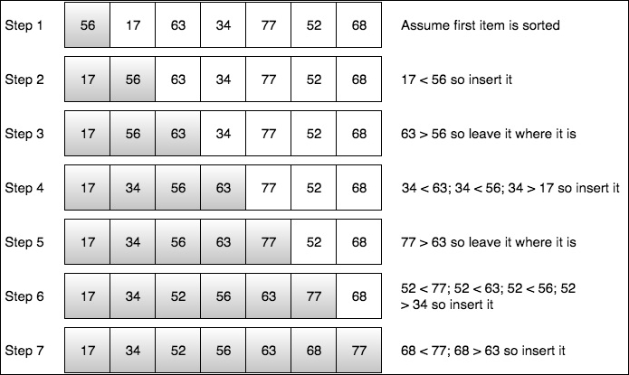
Given the list in Step 1, we assume the first item is in sorted order. In Step 2, we start at the second item and compare it to the previous item, if it is smaller we move the higher item to the right and insert the second item in first position and stop since we're at the beginning. We continue the same pattern in Step 3. In Step 4, it gets a little more interesting. We compare our current item, 34, to the previous one, 63. Since 34 is less than 63, we move 63 to the right. Next, we compare 34 to 56. Since it is also less, we move 56 to the right. Next, we compare 34 to 17, Since 17 is greater than 34, we insert 34 at the current position. We continue this pattern for the remaining steps.

Now let's consider an insertion sort algorithm:

func insertionSort( alist: inout [Int]){ 
    for i in 1..<alist.count { 
        let tmp = alist[i] 
        var j = i - 1 
        while j >= 0 && alist[j] > tmp { 
            alist[j+1] = alist[j] 
            j = j - 1 
        } 
        alist[j+1] = tmp 
    } 
} 

If we call this function with an array of 500, it should be pretty quick. Recall previously where we said the insertion sort represents a quadratic running time where f(x) = c*n²+q. We can express the complexity of this function with the formula, ƒ(x) ϵ O(x²), which means that the function f grows no faster than the quadratic polynomial x², in the asymptotic sense. Often a Big-O notation is abused by making statements such as the complexity of f(x) is O(x²). What we mean is that the worst case f will take O(x²) steps to run. There is a subtle difference between a function being in O(x²) and being O(x²), but it is important. Saying that ƒ(x) ϵ O(x²) does not preclude the worst-case running time of f from being considerably less than O(x²). When we say f(x) is O(x²), we're implying that x² is both an upper and lower bound on the asymptotic worst-case running time.

Let's visualize how merge sort works before we look at the algorithm implementation:

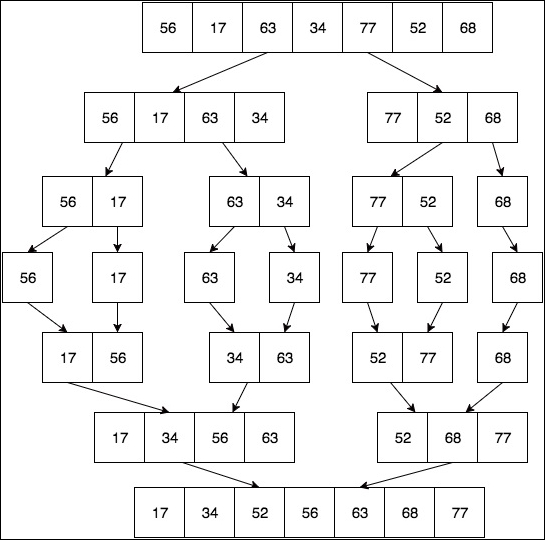
In Chapter 4, Sorting Algorithms, we will take a detailed look at the merge sort algorithm so we'll just take a high-level view of it for now. The first thing we do is begin to divide our array, roughly in half depending on the number of elements. We continue to do this recursively until we have a list size of 1. Then we begin the combine phase by merging the sublists back into a single sorted list.

Now let's consider a merge sort algorithm:

func mergeSort<T:Comparable>(inout list:[T]) { 
    if list.count <= 1 { 
        return 
    } 
     
    func merge(var left:[T], var right:[T]) -> [T] { 
        var result = [T]() 
         
        while left.count != 0 && right.count != 0 { 
            if left[0] <= right[0] { 
                result.append(left.removeAtIndex(0)) 
            } else { 
                result.append(right.removeAtIndex(0)) 
            } 
        } 
         
        while left.count != 0 { 
            result.append(left.removeAtIndex(0)) 
        } 
         
        while right.count != 0 { 
            result.append(right.removeAtIndex(0)) 
        } 
         
        return result 
    } 
     
    var left = [T]() 
    var right = [T]() 
     
    let mid = list.count / 2 
     
    for i in 0..<mid { 
        left.append(list[i]) 
    } 
     
    for i in mid..<list.count { 
        right.append(list[i]) 
    } 
     
    mergeSort(&left) 
    mergeSort(&right) 
     
    list = merge(left, right: right) 
} 

Tip

The source code for insertion sort and merge sort is provided as part of this book's source code download bundle. You can either run it in Xcode Playground or copy/paste it into the Swift REPL to experiment with it.

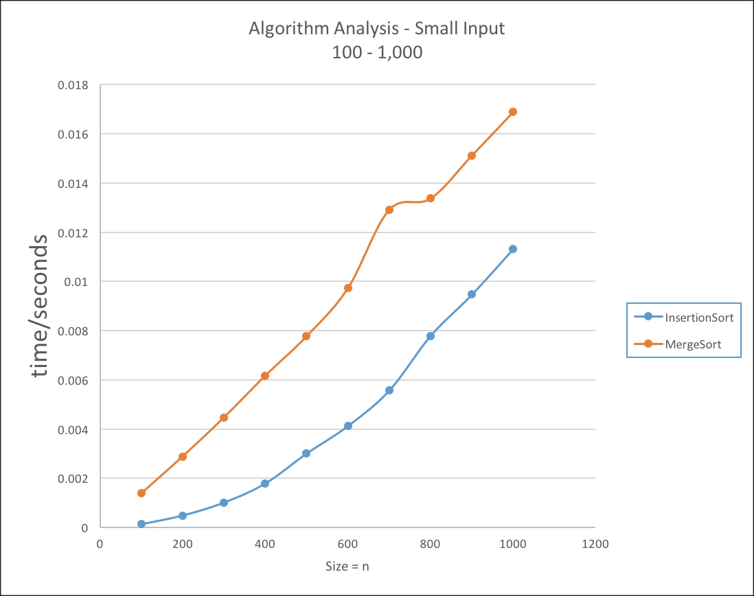
In Table 1.3, we can see with smaller sized inputs it appears at first glance that the insertion sort offers better performance over the merge sort:

Table 1.3 – Small Input Size: 100-1,000 items / seconds

n	T(n2)	Tm(n)
100	0.000126958	0.001385033
200	0.00048399	0.002885997
300	0.001008034	0.004469991
400	0.00178498	0.006169021
500	0.003000021	0.007772028
600	0.004121006	0.009727001
700	0.005564034	0.012910962
800	0.007784009	0.013369977
900	0.009467959	0.01511699
1,000	0.011316955	0.016884029

We can see from the following graph that the insertion sort performs quicker than the merge sort:

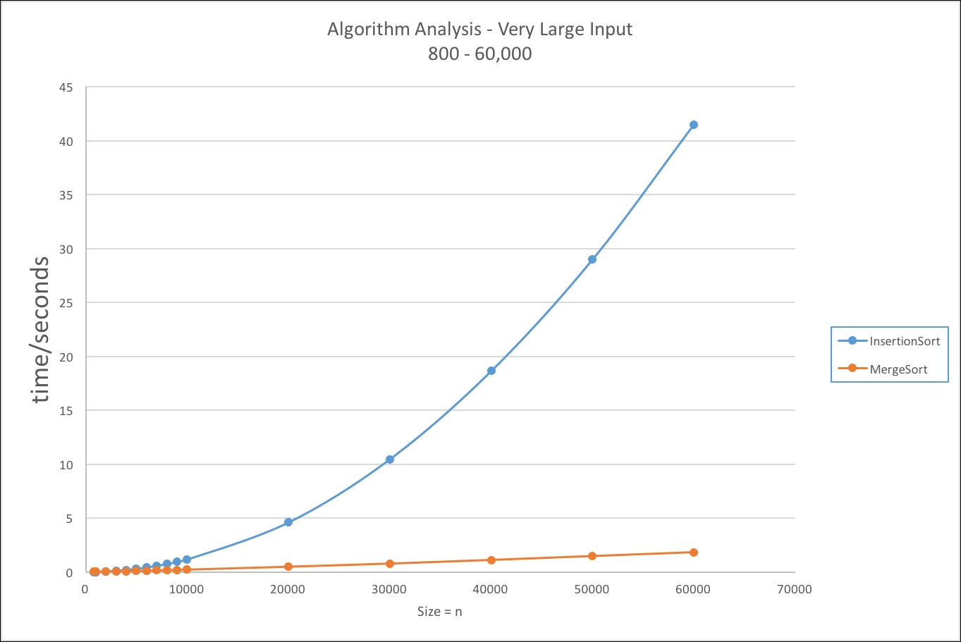
We can see in Table 1.4, what happens as our input gets very large using the insertion sort and merge sort we used previously:

Table 1.4 – Very Large Input Size: 2,000-60,000 items / seconds

n	T(n2)	Tm(n)
800	0.007784009	0.013369977
900	0.009467959	0.01511699
1,000	0.011316955	0.016884029
2,000	0.04688704	0.036652982
3,000	0.105984986	0.05787003
4,000	0.185739994	0.077836037
5,000	0.288598955	0.101580977
6,000	0.417855978	0.124255955
7,000	0.561426044	0.14714098
8,000	0.73259002	0.169996023
9,000	0.930015028	0.197144985
10,000	1.144114017	0.222028017
20,000	4.592146993	0.492881
30,000	10.45656502	0.784195006
40,000	18.64617997	1.122103989
50,000	29.000718	1.481712997
60,000	41.51619297	1.839293003

In this graph, the data clearly shows that the insertion sort algorithm does not scale for larger values of n:

Algorithmic complexity is a very important topic in computer science; this was just a basic introduction to the topic to raise your awareness on the subject. Towards the end of this book, we will cover these topics in greater detail in their own chapter.