Strategies to reduce the data size and improve performance
Using some of the test data that we have generated, or any other data that you might want, we can discover more about how QlikView handles different scenarios. Understanding these different situations will give you real mastery over data load optimization.
Optimizing field values and keys
To begin with, let's see what happens when we load two largish tables that are connected by a key. So, let's ignore the dimension tables and load the order data using a script like the following:
Order:
LOAD OrderID,
     OrderDate,
     CustomerID,
     EmployeeID,
     Freight
FROM
[..\Scripts\OrderHeader.qvd]
(qvd);
OrderLine:
LOAD OrderID,
     LineNo,
     ProductID,
     Quantity,
     SalesPrice,
     SalesCost,
     LineValue,
     LineCost
FROM
[..\Scripts\OrderLine.qvd]
(qvd);
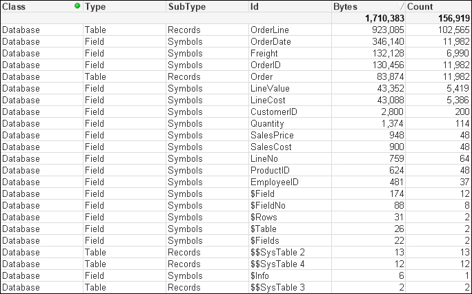
The preceding script will result in a database memory profile that looks like the following. In the following screenshot, Database has been selected for Class:

There are some interesting readings in this table. For example, we can see that when the main data table—OrderLine—is stored with just its pointer records, it takes up just 923,085 bytes for 102,565 records. That is an average of only 9 bytes per record. This shows the space benefit of the bit-stuffed pointer mechanism as described in Henric's blog post.
The largest individual symbol table is the OrderDate field. This is very typical of a TimeStamp field, which will often be highly unique, have long decimal values, and have the Dual text value, and so often takes up a lot of memory—28 bytes per value.
The number part of a TimeStamp field contains an integer representing the date (number of days since 30th December 1899) and a decimal representing the time. So, let's see what happens with this field if we turn it into just an integer—a common strategy with these fields as the time portion may not be important:
Order:
LOAD OrderID,
     Floor(OrderDate) As DateID,
     ...
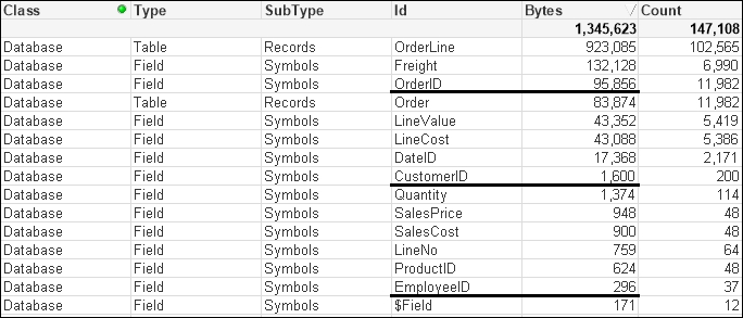
This changes things considerably:

The number of unique values has been vastly reduced, because the highly unique date and time values have been replaced with a much lower cardinality (2171) date integer, and the amount of memory consumed is also vastly reduced as the integer values are only taking 8 bytes instead of the 28 being taken by each value of the TimeStamp field.
The next field that we will pay attention to is OrderID. This is the key field, and key fields are always worth examining to see whether they can be improved. In our test data, the OrderID field is alphanumeric—this is not uncommon for such data. Alphanumeric data will tend to take up more space than numeric data, so it is a good idea to convert it to integers using the AutoNumber function.
AutoNumber accepts a text value and will return a sequential integer. If you pass the same text value, it will return the same integer. This is a great way of transforming alphanumeric ID values into integers. The code will look like the following:
Order:
LOAD AutoNumber(OrderID) As OrderID,
     Floor(OrderDate) As DateID,
   ...

OrderLine:
LOAD AutoNumber(OrderID) As OrderID,
     LineNo,
   ...
This will result in a memory profile like the following:

The OrderID field is now showing as having 0 bytes! This is quite interesting because what QlikView does with a field containing sequential integers is that it does not bother to store the value in the symbol table at all; it just uses the value as the pointer in the data table. This is a great design feature and gives us a good strategy for reducing data sizes.
We could do the same thing with the CustomerID and EmployeeID fields:
Order:
LOAD AutoNumber(OrderID) As OrderID,
     Floor(OrderDate) As DateID,
     AutoNumber(CustomerID) As CustomerID,
     AutoNumber(EmployeeID) As EmployeeID,
     ...
That has a very interesting effect on the memory profile:

Our OrderID field is now back in the Symbols table. The other two tables are still there too. So what has gone wrong?
Because we have simply used the AutoNumber function across each field, now none of them are perfectly sequential integers and so do not benefit from the design feature. But we can do something about this because the AutoNumber function accepts a second parameter—an ID—to identify different ranges of counters. So, we can rejig the script in the following manner:
Order:
LOAD AutoNumber(OrderID, 'Order') As OrderID,
     Floor(OrderDate) As DateID,
     AutoNumber(CustomerID, 'Customer') As CustomerID,
     AutoNumber(EmployeeID, 'Employee') As EmployeeID,
     ...

OrderLine:
LOAD AutoNumber(OrderID, 'Order') As OrderID,
     LineNo,
     ...
This should give us the following result:

This is something that you should consider for all key values, especially from a modeling best practice point of view. There are instances when you want to retain the ID value for display or search purposes. In that case, a copy of the value should be kept as a field in a dimension table and the AutoNumber function used on the key value.
Note
It is worth noting that it is often good to be able to see the key associations—or lack of associations—between two tables, especially when troubleshooting data issues. Because AutoNumber obfuscates the values, it makes that debugging a bit harder. Therefore, it can be a good idea to leave the application of AutoNumber until later on in the development cycle, when you are more certain of the data sources.
Optimizing data by removing keys using ApplyMap
For this example, we will use some of the associated dimension tables—Category and Product. These are loaded in the following manner:
Category:
LOAD CategoryID,
     Category
FROM
[..\Scripts\Categories.txt]
(txt, codepage is 1252, embedded labels, delimiter is '\t', msq);

Product:
LOAD ProductID,
     Product,
     CategoryID,
     SupplierID,
     CostPrice,
     SalesPrice
FROM
[..\Scripts\Products.txt]
(txt, codepage is 1252, embedded labels, delimiter is '\t', msq);
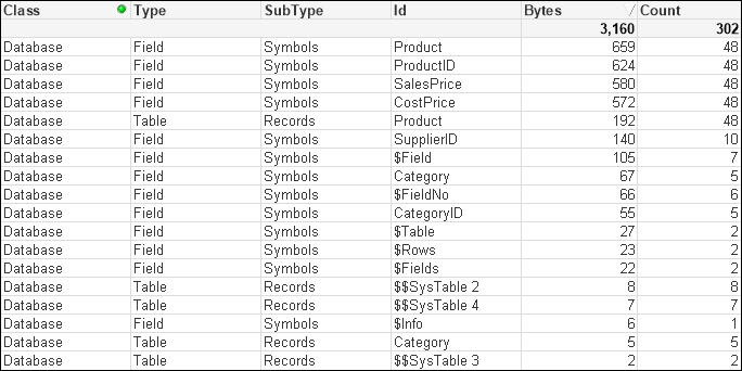
This has a small memory profile:

The best way to improve the performance of these tables is to remove the CategoryID field by moving the Category value into the Product table. When we have small lookup tables like this, we should always consider using ApplyMap:
Category_Map:
Mapping
LOAD CategoryID,
     Category
FROM
[..\Scripts\Categories.txt]
(txt, codepage is 1252, embedded labels, delimiter is '\t', msq);

Product:
LOAD ProductID,
     Product,
     //CategoryID,
     ApplyMap('Category_Map', CategoryID, 'Other') As Category,
     SupplierID,
     CostPrice,
     SalesPrice
FROM
[..\Scripts\Products.txt]
(txt, codepage is 1252, embedded labels, delimiter is '\t', msq);
By removing the Symbols table and the entry in the data table, we have reduced the amount of memory used. More importantly, we have reduced the number of joins required to answer queries based on the Category table:

Optimizing performance by removing keys by joining tables
If the associated dimension table has more than two fields, it can still have its data moved into the primary dimension table by loading multiple mapping tables; this is useful if there is a possibility of many-to-many joins. You do have to consider, however, that this does make the script a little more complicated and, in many circumstances, it is a better idea to simply join the tables.
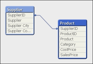
For example, suppose that we have the previously mentioned Product table and an associated Supplier table that is 3,643 bytes:

By joining the Supplier table to the Product table and then dropping SupplierID, we might reduce this down to, say, 3,499 bytes, but more importantly, we improve the query performance:
Join (Product)
LOAD SupplierID,
     Company As Supplier,
     ...

Drop Field SupplierID;
Optimizing memory by removing low cardinality fields
Joining tables together is not always the best approach from a memory point of view. It could be possible to attempt to create the ultimate joined table model of just having one table containing all values. This will work, and query performance should, in theory, be quite fast. However, the way QlikView works is the wider and longer the table you create, the wider and longer the underlying pointer data table will be. Let's consider an example.
Quite often, there will be a number of associated fields in a fact table that have a lower cardinality (smaller number of distinct values) than the main keys in the fact table. A quite common example is having date parts within the fact table. In that case, it can actually be a good idea to remove these values from the fact table and link them via a shared key. So, for example, consider we have an Order table loaded in the following manner:
Order:
LOAD AutoNumber(OrderID, 'Order') As OrderID,
     Floor(OrderDate) As DateID,
     Year(OrderDate) As Year,
     Month(OrderDate) As Month,
     Day(OrderDate) As Day,
     Date(MonthStart(OrderDate), 'YYYY-MM') As YearMonth,
     AutoNumber(CustomerID, 'Customer') As CustomerID,
     AutoNumber(EmployeeID, 'Employee') As EmployeeID,
     Freight
FROM
[..\Scripts\OrderHeader.qvd]
(qvd);
This will give a memory profile like the following:

We can see the values for Year, Month, and Day have a very low count. It is worth noting here that Year takes up a lot less space than Month or Day; this is because Year is just an integer and the others are Dual values that have text as well as numbers.
Let's modify the script to have the date fields in a different table in the following manner:
Order:
LOAD AutoNumber(OrderID, 'Order') As OrderID,
     Floor(OrderDate) As DateID,
     AutoNumber(CustomerID, 'Customer') As CustomerID,
     AutoNumber(EmployeeID, 'Employee') As EmployeeID,
     Freight
FROM
[..\Scripts\OrderHeader.qvd]
(qvd);

Calendar:
Load Distinct
     DateID,
     Date(DateID) As Date,
     Year(DateID) As Year,
     Month(DateID) As Month,
     Day(DateID) As Day,
     Date(MonthStart(DateID), 'YYYY-MM') As YearMonth
Resident
   Order;
We can see that there is a difference in the memory profile:

We have all the same symbol table values that we had before with the same memory. We do have a new data table for Calendar, but it is only quite small because there are only a small number of values. We have, however, made a dent in the size of the Order table because we have removed pointers from it. This effect will be increased as the number of rows increases in the Order table, whereas the number of rows in the Calendar table will not increase significantly over time.
Of course, because the data is now in two tables, there will be a potential downside in that joins will need to be made between the tables to answer queries. However, we should always prefer to have a smaller memory footprint. But how can we tell if there was a difference in performance?


