Solving the Blackjack problem with the Q-learning algorithm
Q-learning is also a model-free learning algorithm. It updates the Q-function for every step in an episode. We will demonstrate how Q-learning is used to solve the Blackjack environment.
Introducing the Q-learning algorithm
Q-learning is an off-policy learning algorithm that optimizes the Q-values based on data generated by a behavior policy. The behavior policy is a greedy policy where it takes actions that achieve the highest returns for given states. The behavior policy generates learning data and the target policy (the policy we attempt to optimize) updates the Q-values based on the following equation:

Here,  is the resulting state after taking action a from state s and r is the associated reward.
  means that the behavior policy generates the highest Q-value given state
  . Hyperparameters
  and
and  are the learning rate and discount factor respectively. The Q-learning equation updates the Q-value (estimated future reward) of a state-action pair based on the current Q-value, the immediate reward, and the potential future rewards the agent can expect by taking the best possible action in the next state.
Learning from the experience generated by another policy enables Q-learning to optimize its Q-values in every single step in an episode. We gain the information from a greedy policy and use this information to update the target values right away.
One more thing to note is that the target policy is epsilon-greedy, meaning it takes a random action with a probability of  (value from 0 to 1) and takes a greedy action with a probability of
  . The epsilon-greedy policy combines exploitation and exploration: it exploits the best action while exploring different actions.
Developing the Q-learning algorithm
Now it is time to develop the Q-learning algorithm to solve the Blackjack environment:
- We start with defining the epsilon-greedy policy:
>>> def epsilon_greedy_policy(n_action, epsilon, state, Q):
...     probs = torch.ones(n_action) * epsilon / n_action
...     best_action = torch.argmax(Q[state]).item()
...     probs[best_action] += 1.0 - epsilon
...     action = torch.multinomial(probs, 1).item()
...     return action
Given  possible actions, each action is taken with a probability
  , and the action with the highest state-action value is chosen with an additional probability
  .
.
- We will start with a large exploration factor
 and reduce it over time until it reaches
 0.1. We define the starting and final as follows:
>>> epsilon = 1.0 >>> final_epsilon = 0.1 - Next, we implement the Q-learning algorithm:
>>> def q_learning(env, gamma, n_episode, alpha, epsilon, final_epsilon):
        n_action = env.action_space.n
        Q = defaultdict(lambda: torch.zeros(n_action))
        epsilon_decay = epsilon / (n_episode / 2)
        for episode in range(n_episode):
            state, _ = env.reset()
            is_done = False
            epsilon = max(final_epsilon, epsilon - epsilon_decay)
            while not is_done:
                action = epsilon_greedy_policy(n_action, epsilon, state, Q)
                next_state, reward, terminated, truncated, info = env.step(action)
                is_done = terminated or truncated
                delta = reward + gamma * torch.max(
                                           Q[next_state]) - Q[state][action]
                Q[state][action] += alpha * delta
                total_reward_episode[episode] += reward
                if is_done:
                    break
                state = next_state
        policy = {}
        for state, actions in Q.items():
            policy[state] = torch.argmax(actions).item()
        return Q, policy
We initialize the action-value function Q and calculate the epsilon decay rate for the epsilon-greedy exploration strategy. For each episode, we let the agent take actions following the epsilon-greedy policy, and update the Q function for each step based on the off-policy learning equation. The exploration factor also decreases over time. We run n_episode episodes and finally extract the optimal policy from the learned action-value function Q by selecting the action with the maximum value for each state.
- We then initiate a variable to store the performance of each of 10,000 episodes, measured by the reward:
>>> n_episode = 10000 >>> total_reward_episode = [0] * n_episode - Finally, we perform Q-learning to obtain the optimal policy for the Blackjack problem with the following hyperparameters:
>>> gamma = 1
>>> alpha = 0.003
>>> optimal_Q, optimal_policy = q_learning(env, gamma, n_episode, alpha,
                                           epsilon, final_epsilon)
Here, discount rate  and learning rate
  for more exploration.
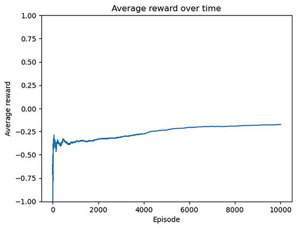
- After 10,000 episodes of learning, we plot the rolling average rewards over the episodes as follows:
>>> rolling_avg_reward = [total_reward_episode[0]]
>>> for i, reward in enumerate(total_reward_episode[1:], 1):
        rolling_avg_reward.append((rolling_avg_reward[-1]*i + reward)/(i+1))
>>> plt.plot(rolling_avg_reward)
>>> plt.title('Average reward over time')
>>> plt.xlabel('Episode')
>>> plt.ylabel('Average reward')
>>> plt.ylim([-1, 1])
>>> plt.show()
Refer to the following screenshot for the end result:

Figure 15.5: Average reward over episodes
The average reward steadily rises throughout the training process, eventually converging. This indicates that the model becomes proficient in solving the problem after training.
- Finally, we simulate 100,000 episodes for the optimal policy we obtained using Q-learning and calculate the winning chance:
>>> n_episode = 100000
>>> n_win_opt = 0
>>> for _ in range(n_episode):
...     reward = simulate_episode(env, optimal_policy)
...     if reward == 1:
...         n_win_opt += 1
>>>print(f'Winning probability under the optimal policy: {n_win_opt/n_episode}')
Winning probability under the optimal policy: 0.42398
Playing under the optimal policy has a 42% chance of winning.
In this section, we solved the Blackjack problem with off-policy Q-learning. The algorithm optimizes the Q-values in every single step by learning from the experience generated by a greedy policy.


