Search icon CANCEL
Subscription
0
Cart icon
Your Cart (0 item)
Close icon
You have no products in your basket yet
Save more on your purchases! discount-offer-chevron-icon
Savings automatically calculated. No voucher code required.
Arrow left icon
Explore Products
Best Sellers
New Releases
Books
Videos
Audiobooks
Learning Hub
Free Learning
Arrow right icon
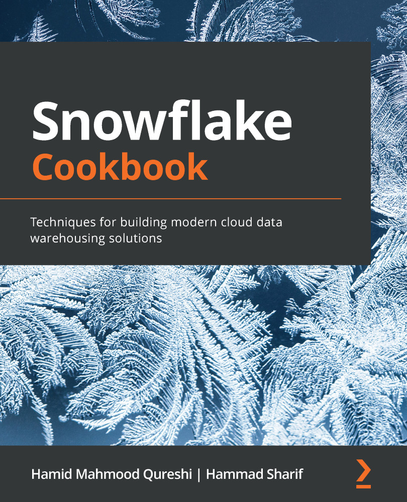
Snowflake Cookbook
Snowflake Cookbook

Snowflake Cookbook: Techniques for building modern cloud data warehousing solutions

Arrow left icon
Profile Icon Hamid Mahmood Qureshi Profile Icon Hammad Sharif
Arrow right icon
€37.99
Full star icon Full star icon Full star icon Full star icon Half star icon 4.2 (17 Ratings)
Paperback Feb 2021 330 pages 1st Edition
eBook
€8.99 €29.99
Paperback
€37.99
Subscription
Free Trial
Renews at €18.99p/m
eBook
€8.99 €29.99
Paperback
€37.99
Subscription
Free Trial
Renews at €18.99p/m

What do you get with Print?

Product feature icon Instant access to your digital eBook copy whilst your Print order is Shipped
Product feature icon Paperback book shipped to your preferred address
Product feature icon Download this book in EPUB and PDF formats
Product feature icon Access this title in our online reader with advanced features
Product feature icon DRM FREE - Read whenever, wherever and however you want
Product feature icon AI Assistant (beta) to help accelerate your learning
OR
Modal Close icon
Payment Processing...
tick Completed

Shipping Address

Billing Address

Shipping Methods
Table of content icon View table of contents Preview book icon Preview Book

Snowflake Cookbook

Chapter 2: Managing the Data Life Cycle

This chapter provides a set of recipes that introduce you to data management in Snowflake. The chapter talks about common database concepts and introduces you to nuances specific to Snowflake. We'll look at common operations that are required to manage and structure data in a database. Snowflake is not very different from traditional databases and provides similar capabilities, but since Snowflake has been designed for the cloud from the ground up, it has small configurations that allow control over how data is managed in a database or a table and how temporary data is maintained and destroyed when not required. These capabilities are required when designing an ETL system or structuring data according to a data model.

The following recipes are given in this chapter:

  • Managing a database
  • Managing a schema
  • Managing tables
  • Managing external tables and stages
  • Managing views in Snowflake

Technical requirements

The chapter assumes that you have a Snowflake account already set up. It also requires you to have access to an Amazon S3 bucket to use to get hold of external data and use it within Snowflake.

The code for this chapter can be found at the following GitHub URL:

https://github.com/PacktPublishing/Snowflake-Cookbook/tree/master/Chapter02

Managing a database

In this recipe, we will create a new database with default settings and walk through several variations on the database creation process. The recipe provides details such as how to minimize storage usage when creating databases and how to set up the replication of databases across regions and when to do so.

Getting ready

This recipe describes the various ways to create a new database in Snowflake. These steps can be run either in the Snowflake web UI or the SnowSQL command-line client.

How to do it…

Let's start with the creation of a database in Snowflake:

  1. The basic syntax for creating a new database is fairly straightforward. We will be creating a new database that is called our_first_database. We are assuming that the database doesn't exist already:
    CREATE DATABASE our_first_database
    COMMENT = 'Our first database';

    The command should successfully execute with the following message:

    Figure 2.1 – Database successfully created

    Figure 2.1 – Database successfully created

  2. Let's verify that the database has been created successfully and review the defaults that have been set up by Snowflake:
    SHOW DATABASES LIKE 'our_first_database';

    The query should return one row showing information about the newly created database, such as the database name, owner, comments, and retention time. Notice that retention_time is set to 1 and the options column is blank:

    Figure 2.2 – Information of the newly created database

    Figure 2.2 – Information of the newly created database

  3. Let's create another database for which we will set the time travel duration to be 15 days (in order to set the time travel duration above 1 day, you must have at least the Enterprise license for Snowflake):
    CREATE DATABASE production_database 
    DATA_RETENTION_TIME_IN_DAYS = 15
    COMMENT = 'Critical production database';
    SHOW DATABASES LIKE 'production_database';

    The output of SHOW DATABASES should now show retention_time as 15, indicating that the time travel duration for the database is 15 days:

    Figure 2.3 – SHOW DATABASES output

    Figure 2.3 – SHOW DATABASES output

  4. While time travel is normally required for production databases, you wouldn't normally need time travel and the fail-safe for temporary databases such as databases that are used in ETL processing. Removing time travel and the fail-safe helps in reducing storage costs. Let's see how that is done:
    CREATE TRANSIENT DATABASE temporary_database 
    DATA_RETENTION_TIME_IN_DAYS = 0
    COMMENT = 'Temporary database for ETL processing';
    SHOW DATABASES LIKE 'temporary_database';

    The output of SHOW DATABASES would show retention_time as zero, indicating that there is no time travel storage for this database, and also the options column would show TRANSIENT as the option, which essentially means that there will be no fail-safe storage for this database.

  5. The time travel configuration can also be changed at a later time by altering the database with ALTER:
    ALTER DATABASE temporary_database
    SET DATA_RETENTION_TIME_IN_DAYS = 1;
    SHOW DATABASES LIKE 'temporary_database';

How it works…

The basic CREATE DATABASE command creates a database with the defaults set at the account level. If you have not changed the defaults, the default for time travel is 1 day, which is the value that appears in retention_time when you run the SHOW DATABASES command. The database will also have a fail-safe enabled automatically. Both these options will cost you in storage, and in certain cases, you might want to reduce those storage costs. As an example, databases that are used for temporary ETL processing can easily be configured to avoid these costs.

A key thing to know about databases and tables used for ETL processing is that the data in those tables will be repeatedly inserted and deleted. If such tables are not specifically configured, you will be unnecessarily incurring costs for the time travel and fail-safe that is stored with every data change that happens for those tables. We will set such databases to be transient (with TRANSIENT) so that the fail-safe option is not the default for the tables in that database. Setting this option does mean that such databases are not protected by fail-safe if a data loss event occurs, but for temporary databases and tables, this should not be an issue. Also, we have set time travel to be zero so that there is no time travel storage as well.

Do note that although we have set the database to have no time travel and no fail-safe, we can still set individual tables within the database to be protected by the fail-safe and time travel. Setting these options at the database level only changes the defaults for the objects created within that database.

Note that there is the ALTER DATABASE command as well, which can be used to change some of the properties after the database has been created. It is a powerful command that allows renaming the database, swapping a database with another database, and also resetting custom properties back to their defaults.

It is important to note that creating a database sets the current database of the session to the newly created database. That would mean that any subsequent data definition language (DDL) commands such as CREATE TABLE would create a table under that new database. This is like using the USE DATABASE command.

There's more…

We will cover time travel and fail-safes in much more detail in subsequent chapters. We will also cover in depth how to create databases from shares and databases that clone other databases.

Managing a schema

In this recipe, you will be introduced to the concept of a schema and its uses. A schema is a counterpart of a database, and together, these two define a namespace. There can be multiple schemas in a database, but one schema belongs to a single database. Schemas help in grouping tables and views together that are logically related. We will see how a schema is created and its use. Apart from user-created schemas, we will learn about schemas that are automatically available with a database, including the information schema provided by Snowflake.

Getting ready

The following examples can be run either via the Snowflake web UI or the SnowSQL command-line client.

How to do it…

Let's start with the creation of a user-defined schema in a user-defined database, followed by the listing of schemas:

  1. Let's first create a database in which we will test the schema creation:
    CREATE DATABASE testing_schema_creation;

    You should see a message stating that a schema was successfully created:

    Figure 2.4 – Database created successfully

    Figure 2.4 – Database created successfully

  2. Let's check whether the newly created database already has a schema in it:
    SHOW SCHEMAS IN DATABASE testing_schema_creation;

    You should see two rows in the result set, which are basically the two schemas that are automatically available with every new database:

    Figure 2.5 – Schemas of the new database

    Figure 2.5 – Schemas of the new database

  3. Let's now create a new schema. The syntax for creating a standard schema without any additional settings is quite simple, as shown in the following SQL code:
    CREATE SCHEMA a_custom_schema
    COMMENT = 'A new custom schema';

    The command should successfully execute with the following message:

    Figure 2.6 – New schema successfully created

    Figure 2.6 – New schema successfully created

  4. Let's verify that the schema has been created successfully and also look at the default values that were set automatically for its various attributes:
    SHOW SCHEMAS LIKE 'a_custom_schema' IN DATABASE testing_schema_creation ;

    The query should return one row displaying information such as the schema name, the database name in which the schema resides, and the time travel retention duration in days:

    Figure 2.7 – Validating the schema

    Figure 2.7 – Validating the schema

  5. Let's create another schema for which we will set the time travel duration to be 0 days and also set the type of the schema to be transient. It is common to use these settings on data for which Snowflake data protection features are not required, such as temporary data:
    CREATE TRANSIENT SCHEMA temporary_data 
    DATA_RETENTION_TIME_IN_DAYS = 0
    COMMENT = 'Schema containing temporary data used by ETL processes';

    The schema creation should succeed with the following message:

    Figure 2.8 – New schema successfully created

    Figure 2.8 – New schema successfully created

  6. Let's view what the schema settings are by running a SHOW SCHEMAS command as shown:
    SHOW SCHEMAS LIKE 'temporary_data' IN DATABASE testing_schema_creation ;

    The output of SHOW SCHEMAS is shown here:

Figure 2.9 – Output of SHOW SCHEMAS

Figure 2.9 – Output of SHOW SCHEMAS

The output should show retention_time as zero or a blank value, indicating that there is no time travel storage for this schema, and also the options column should show TRANSIENT as the option, which essentially means that there will be no fail-safe storage for this schema.

How it works…

The standard CREATE SCHEMA command uses the defaults set at the database level. If you have not changed any of the configuration, the created schema will have fail-safe enabled by default. Also, time travel is enabled for the schema automatically and is set to be 1 day by default. Both these features have costs associated with them and in certain cases, you can choose to turn off these features.

For schemas that will store temporary tables, such as tables used for ETL processing, a schema can be created as a transient schema, which means that there is no fail-safe storage associated with the tables created in the schema, and therefore it would cost less. Similarly, such schemas can also be set to have time travel set to zero to reduce costs further. By default, the time travel for transient schemas is 1 day.

Do note that although we have set the schema to have no time travel and no fail-safe, we can still set individual tables within the schema to be protected by fail-safe and time travel. Setting these options at the schema level sets the default for all tables created inside that schema.

It is important to note that creating a new schema sets the current schema of the session to the newly created schema. The implication of this behavior is that any subsequent DDL commands such as CREATE TABLE would create the table under that new schema. This is like issuing the USE SCHEMA command to change the current schema.

There's more…

Every database in Snowflake will always have a public schema that is automatically created upon database creation. Additionally, under every database, you will also find an additional schema called the information schema. The information schema implements the SQL 92 standard information schema and adds additional information specific to Snowflake. The purpose of the information schema is to act as a data dictionary containing metadata that you can query to find information such as all the tables in the system, all columns along with their data types, and more. It is possible to add many additional schemas under a given database, which can help you organize your tables in a meaningful structure.

A good example of using databases and schemas to organize your data and your environment would be the approach of setting up production, testing, and development databases using the concept of schemas and databases. This approach is especially required if your organization has a single Snowflake account that is being used for development, testing, and production purposes at the same time. The approach is shown in the following diagram:

Figure 2.10 – A DEV, TEST, PROD setup using databases and schemas

Figure 2.10 – A DEV, TEST, PROD setup using databases and schemas

In this approach, a database is created for each environment, for example, the PROD database for production data, the DEV database for development data, and so on. Within each database, the schema structures are identical; for example, each database has an SRC schema, which contains the source data. The purpose of this approach is to segregate the various environments but keep the structures identical enough to facilitate the development, testing, and productionization of data.

Managing tables

This recipe shows you how to create a table and insert data to explain different behaviors in storing data. Here you will be introduced to the different options that are available from a life cycle perspective, such as tables being permanent, temporary, volatile, and so on. Most of the concepts are not new, so the focus is going to be on the specifics related to Snowflake. We will start with a simple example that creates a table. We shall insert some sample data into it and then try out different variations on creating tables in Snowflake.

Getting ready

The following examples can be run either via the Snowflake web UI or the SnowSQL command-line client.

How to do it…

Let's start by creating a table for storing customer data. We shall start with the DDL statement for creating a table:

  1. The following example DDL statement will be executed to create a table called CUSTOMERS in Snowflake:
    CREATE TABLE customers (
      id              INT NOT NULL,
      last_name       VARCHAR(100) ,
      first_name      VARCHAR(100),
      email           VARCHAR(100),
      company         VARCHAR(100),
      phone           VARCHAR(100),
      address1        VARCHAR(150),
      address2        VARCHAR(150),
      city            VARCHAR(100),
      state           VARCHAR(100),
      postal_code     VARCHAR(15),
      country         VARCHAR(50)
    );

    The command should successfully execute, generating the following message:

    Figure 2.11 – Table created successfully

    Figure 2.11 – Table created successfully

  2. To confirm that the table has been generated as per the specification, we can run a DESCRIBE TABLE statement a shown:
    DESCRIBE TABLE customers;

    It should generate the following results in the Snowflake web UI:

    Figure 2.12 –  Output of the DESCRIBE statement

    Figure 2.12 – Output of the DESCRIBE statement

  3. Let's assume there was something wrong with a data type; for example, say ADDRESS1 and ADDRESS2 were supposed to be stored as a STRING data type. This can be addressed using the REPLACE TABLE statement, along with CREATE. This will overwrite the existing CUSTOMERS table:
    CREATE TABLE customers (
      id              INT NOT NULL,
      last_name       VARCHAR(100) ,
      first_name      VARCHAR(100),
      email           VARCHAR(100),
      company         VARCHAR(100),
      phone           VARCHAR(100),
      address1        STRING,
      address2        STRING,
      city            VARCHAR(100),
      state           VARCHAR(100),
      postal_code     VARCHAR(15),
      country         VARCHAR(50)
    );
  4. Let's verify whether the desired change has been successfully applied. For that, we can execute the DESCRIBE TABLE statement again as shown:
    DESCRIBE TABLE customers;

    It should generate the following result in the Snowflake web UI:

    Figure 2.13 – Output of the DESCRIBE statement after the changes in the table

    Figure 2.13 – Output of the DESCRIBE statement after the changes in the table

    Please note the data types. We shall discuss this in the How it works… section along with how REPLACE works and how it is a shorthand for a two-step process typically required for managing the life cycle of a table.

  5. Let's now load this table with some data before we continue with the rest of the recipe. To do so, run the following command:
    COPY INTO customers
    FROM s3://snowflake-cookbook/Chapter02/r3/customer.csv
    FILE_FORMAT = (TYPE = csv SKIP_HEADER = 1 FIELD_OPTIONALLY_ENCLOSED_BY = '"');

    This should complete with the following message:

    Figure 2.14 – Table loaded

    Figure 2.14 – Table loaded

  6. Let's now look at scenarios where the creation of a table is based on an existing table. A common pattern in the table life cycle involves deriving a table from an existing table. This is called CTAS or CREATE TABLE ... AS SELECT. To explain the use of CTAS, we will have some records inserted into the CUSTOMERS table. The dataset has 100 rows, as shown in the following screenshot (showing the first six columns of the table):
    Figure 2.15 – Sample data shown for the customer table

    Figure 2.15 – Sample data shown for the customer table

  7. The dataset will be copied into a new table that will have the same structure as the CUSTOMERS table. The statements to be executed are as follows:
    CREATE OR REPLACE TABLE 
    customers_deep_copy 
    AS 
    SELECT * 
    FROM customers;

    This should succeed with the following message:

    Figure 2.16 – Deep copy table created

    Figure 2.16 – Deep copy table created

    What we now have created is a deep copy of the CUSTOMERS table and a new table, which has received all data from CUSTOMERS and is called CUSTOMERS_DEEP_COPY. The deep copy means that the table structure and data has been copied, as opposed to a shallow copy, which would copy the table structure only. This copied table is now an independent copy that can have a life cycle of its own with no changes or side effects originating from any operations performed on the CUSTOMERS table. A SELECT QUERY statement on this new table would generate the same results as shown in the previous table.

  8. Now let's look at another table copying method – shallow copy. In certain situations, a new table is required to be created with the same structure as an existing table, but the data is not to be copied, in which case a shallow copy is created. This is achieved by using the LIKE keyword as provided by Snowflake:
    CREATE OR REPLACE TABLE 
    customers_shallow_copy 
    LIKE customers;

    This should succeed with the following message:

    Figure 2.17 – Shallow copy table created

    Figure 2.17 – Shallow copy table created

  9. This should create a table that has the same structure as the CUSTOMERS table but with no data in it:
    SELECT 
    COUNT(*)
    FROM 
    customers_shallow_copy;

    The result of the following count query is 0 rows, as shown:

    Figure 2.18 – New empty table created

    Figure 2.18 – New empty table created

  10. Until now, we have seen the creation of tables with permanent life – the table will exist and store data until explicitly dropped. This is the default behavior from a life cycle perspective. There are tables that handle transitory data and so they might be required only temporarily. For such scenarios, there are temporary and transient tables. Let's create these tables by running the following SQL statements:
    CREATE TEMPORARY TABLE customers_temp AS SELECT * FROM customers WHERE TRY_TO_NUMBER(postal_code) IS NOT NULL;
    CREATE TRANSIENT TABLE customers_trans AS AS SELECT * FROM customers WHERE TRY_TO_NUMBER(postal_code) IS NULL;
  11. The preceding SQL script will allow you to create two tables, customers_temp and customers_trans. The two tables are not permanent, but the tables have limitations. If you end the web UI session at this point, then the customers_temp table will not be recoverable after a re-login. Transient tables are available after a session has been closed and will retain data in a subsequent session created by user login; however, they don't consume fail-safe storage. This is an important mechanism for retaining data across sessions and can have applications in scenarios that require state management or in ETL jobs.

How it works…

REPLACE is actually a shorthand for a two-step process that's required when a table has to be deleted (dropped) and then recreated. That would typically be done by executing the two statements in sequence as follows:

DROP TABLE IF EXISTS
CREATE TABLE customers …

The deep and shallow copies can be explained by the following query and the result generated by Snowflake:

show tables like 'customers%';

This shows a table with three rows, each showing a summary of the three tables that we have generated previously, explaining the differences and similarities. The following table shows that the deep copies of the dataset are exactly the same while the shallow copy has been deprived of data, though the metadata is the same:

Figure 2.19 – The show tables command output showing the copies of the table

Figure 2.19 – The show tables command output showing the copies of the table

A thing to note in the preceding table is the kind column. The column is showing that the tables created have the kind attribute set as TABLE, which is the default type of table – a permanent table structure to be populated with data rows. (Please note that a select set of columns is being shown here for the sake of clarity.)

A local temporary table (also known as a volatile table) persists for the duration of the user session in which it was created and is not visible to other users. A temporary table's definition and contents are dropped at the end of the user session.

Transient tables are non-permanent tables, but unlike temporary tables, transient tables exist until explicitly dropped and are visible to any user with the appropriate privileges. Transient tables have a lower level of data protection than permanent tables. Data in a transient table may be lost in the event of a system failure. Transient tables should only be used for data that can be recreated in the event that the data is lost.

A show tables command for the customers_temp and customers_trans tables will show a table similar to the following table (please note that a limited set of columns is shown here for the sake of clarity):

Figure 2.20 – The show tables command output highlighting the temporary 
and transient nature of tables

Figure 2.20 – The show tables command output highlighting the temporary and transient nature of tables

Please note the content for the kind column. It shows that the tables are not permanent.

There's more…

One aspect of CREATE TABLE statements, CLONE, has been left for discussion in Chapter 8, Back to the Future with Time Travel. Temporary tables, however, cannot be cloned. Only permanent tables are fail-safe. Fail-safes will be discussed further in later chapters.

Managing external tables and stages

An important aspect of ETL applications is managing the loading of data. This recipe introduces you to managing incoming data by creating a stage and querying that data for loading into native Snowflake tables. The process is very different from traditional data warehouses as it mixes concepts from modern big data systems. Details around ETL will not be covered here but are deferred till later chapters to explain how an ETL pipeline can be managed.

Getting ready

The following example requires SnowSQL to run the different steps. Apart from that, you will need to have access to an AWS S3 bucket where data can be placed and made available as files.

How to do it…

The following steps start with the creation of a stage, which is used to temporarily store data before it can be copied into Snowflake:

  1. Let's first create a stage. A stage is a logical concept or an abstraction of a filesystem location that is external or internal to Snowflake. In this case, an external stage has been used. The location can be managed in one of the object stores supported by the underlying cloud storage. In the case of AWS, S3 is used for this purpose. This recipe uses S3. The following statement creates a stage named sfuser_ext_stage. The stage should be accessible to Snowflake:
    CREATE OR REPLACE STAGE sfuser_ext_stage
    URL='s3://snowflake-cookbook/Chapter02/r4/';

    The response should say that a stage has been created successfully, as shown:

    Figure 2.21 – Stage area created

    Figure 2.21 – Stage area created

  2. Let's now do a listing on the SFUSER_EXT_STAGE stage pointing to the snowflake-cookbook S3 bucket:
    LIST@SFUSER_EXT_STAGE;

     This statement should generate the following output in the web UI:

    Figure 2.22 – Listing the stage to the S3 bucket

    Figure 2.22 – Listing the stage to the S3 bucket

    We can see that there are two types of files in the preceding listing: csv and parquet. In the case of csv, the electronic-card-transactions-may-2020-headless.csv file is a header-less version of the electronic-card-transactions-may-2020.csv file. There is a parquet format file as well called userdata1.parquet. We shall create external tables on both files. An external table is different from usual database tables because unlike tables that point to data inside a database, external tables provide a view on top of files stored in a stage.

    These are read-only tables that maintain metadata that's helpful in interpreting the contents of a file, which could be formatted as parquet, csv, and so on.

  3. Let's now look at how the parquet file can be loaded into an external table. We shall be creating an external table called ext_tbl_userdata1. The creation of the table would require a location from which data can be read into the table. It would also require a file format. In this case, the file type is parquet:
    create or replace external table ext_tbl_userdata1
    with location = @sfuser_ext_stage                                                                      
    file_format = (type = parquet);
  4. Let's query the newly created external table. This would show each row of the result set as a JSON document. Within each row, you should be able to see different columns with their respective values as key-value pairs:
    select * from ext_tbl_userdata1;

    The following screenshot is only showing some of the key-value pairs due to size constraints:

    Figure 2.23 – Output of the query showing key-value pairs

    Figure 2.23 – Output of the query showing key-value pairs

  5. Similarly, by pointing to a different location, the CSV file can be loaded into another external table. An ext_card_data table is created that has the location pointing to the stage. In this case, the file is located in a …/ch2/r4/csv subfolder. This gets us to the folder where the file is located. file_format, in this case, is providing the information that the file is a CSV, and finally, a file filter is provided to constrain the search to CSVs with headless in their names:
    create or replace external table ext_card_data
    with location = @sfuser_ext_stage/csv
    file_format = (type = csv)
    pattern = '.*headless[.]csv';
  6. Let's query the new external table:
    select * from ext_card_data; 

    The following screenshot of the resulting records shows some of the rows generated by the query. Please note the difference here. There are no meaningful column names in this case, unlike the previous case of the Parquet file:

    Figure 2.24 – Output of the select statement

    Figure 2.24 – Output of the select statement

  7. As we have observed, an external table always ends up having data in JSON format at the end of a copy process. This step shows how some meaningful names can be given to the dummy or automatically created columns in the JSON document and how it can be flattened to generate column-oriented rows. The following query shows how aliases can be created for the automatically created column names. Please note that the query only selects two columns, c3 and c2, and creates the card_sum and period aliases, respectively. Moreover, to use the columns effectively, casting has been carried out for each column value:
    select top 5 value:c3::float as card_sum,
    value:c2::string as period 
    from ext_card_data;

    The result of the query is shown:

    Figure 2.25 – Output of the query selecting two columns

    Figure 2.25 – Output of the query selecting two columns

  8. Now that we have loaded tables and we can see how this data can be used in queries, we can drop the tables. This would end the life of the external tables that had been created to run queries of raw data – a typical purge-on-load pattern is applicable:
    drop table ext_card_data;
    drop table ext_tbl_userdata1; 

How it works…

The stage created in step 1 can be thought of as a reference to a storage location. It is treated as a read-only location that can only be accessed using the appropriate access rights. The S3 bucket in step 1 is a public bucket and does not need credentials to be accessed. In later chapters, when we look at staging in more detail, we shall start delving into securing the staging locations.

Step 2 is dereferencing the specified S3 bucket to list all the files that are available along with the last modified dates.

In step 3, when the Parquet file is loaded into the external table, the table rows have all the field names captured, as shown in step 4. But in step 5, when the CSV-formatted file is loaded into the external table, there are dummy column names created by Snowflake, as can be seen in step 6. This is because a Parquet file has metadata stored inside the file, while a CSV file does not have that metadata embedded in it. This is a major difference and would usually require additional steps as shown in step 7 to generate meaningful column names, plus the casting of data types.

There's more…

In this recipe, we did not look at how data could be loaded into a stage. It is possible to load data into a stage from a local filesystem. This method will be discussed in the later chapters.

Looking at the metadata limitations for external tables, it can be argued that Avro files can be the best format for staging data as Avro files can specify field names and data types as well. We shall look into an example in a later chapter where we discuss ETL processing.

Please note that the last modified dates for each file in a stage can be a useful mechanism to trigger updating data in an external table and can be used for running the ETL process.

Managing views in Snowflake

This recipe will introduce you to different variations of views that are specific to Snowflake and in what scenario a variant of a view should be used. The recipe will cover simple views and materialized views and will provide guidance on when to use what type of view.

Getting ready

The following examples can be run either via the Snowflake web UI or the SnowSQL command-line client. Please make sure that you have access to the SNOWFLAKE_SAMPLE_DATA database in your Snowflake instance. The SNOWFLAKE_SAMPLE_DATA database is a database that is shared by Snowflake automatically and provides sample data for testing and benchmarking purposes.

How to do it…

Let's start with the creation of views in Snowflake. We shall look into the creation of simple views on tables and then talk about materialized views:

  1. The SNOWFLAKE_SAMPLE_DATA database contains a number of schemas. We will be making use of the schema called TPCH_SF1000. Within this schema, there are multiple tables, and our view will make use of the STORE_SALES table to produce an output that shows the sales against order dates. Before we create our first view, let's create a database where we will create the views:
    CREATE DATABASE test_view_creation;
  2. Create the view called date_wise_profit that, as the name suggests, shows the profit against the date:
    CREATE VIEW test_view_creation.public.date_wise_orders
    AS
    SELECT L_COMMITDATE AS ORDER_DATE,
    SUM(L_QUANTITY) AS TOT_QTY,
    SUM(L_EXTENDEDPRICE) AS TOT_PRICE
    FROM SNOWFLAKE_SAMPLE_DATA.TPCH_SF1000.LINEITEM
    GROUP BY L_COMMITDATE;

    The view is successfully created with the following message:

    Figure 2.26 – View created successfully

    Figure 2.26 – View created successfully

  3. Let's select some data from this view:
    SELECT * FROM test_view_creation.public.date_wise_orders; 

    The view will take some time (2-3 minutes) to execute as there is a large amount of data in the underlying tables. This latency in execution can be managed by opting for a larger warehouse. An extra-small warehouse has been used in this case. After some time, you should see the result set returned (as shown in the following screenshot), which will be approximately 2,500 rows:

    Figure 2.27 – Selecting data from the view

    Figure 2.27 – Selecting data from the view

  4. Selecting data from this view, as you will have noticed, took a reasonable amount of time to execute, and this time would increase if the amount of data in the table increased over time. To optimize performance, you can choose to create this view as a materialized view. Please note that you will require at least an Enterprise license of Snowflake in order to create materialized views:
    CREATE MATERIALIZED VIEW test_view_creation.public.date_wise_orders_fast
    AS
    SELECT L_COMMITDATE AS ORDER_DATE,
    SUM(L_QUANTITY) AS TOT_QTY,
    SUM(L_EXTENDEDPRICE) AS TOT_PRICE
    FROM SNOWFLAKE_SAMPLE_DATA.TPCH_SF1000.LINEITEM
    GROUP BY L_COMMITDATE;

    The first thing that you will notice when creating the materialized view is that it will not be immediate:

    Figure 2.28 – Creating a materialized view

    Figure 2.28 – Creating a materialized view

    It will take a fair bit of time to create the view as opposed to the immediate creation that we saw in step 2, mainly because materialized views store data, unlike normal views, which just store the DDL commands and fetch data on the fly when the view is referenced.

  5. Let's now select from the materialized view:
    SELECT * FROM test_view_creation.public.date_wise_orders_fast;

    The results are returned almost immediately as we are selecting from a materialized view, which performs much better than a simple view.

How it works…

A standard view in Snowflake is a way to treat the result of a query as if it were a table. The query itself is part of the view definition. When data is selected from a standard view, the query in the view definition is executed and the results are presented back as a table to the user. Since the view appears as a table, it can be joined with other tables as well and used in queries in most places where tables can be used. Views are a powerful method to abstract complex logic from the users of data; that is, a reusable query with complex logic can be created as a view. As such, this takes the burden off the end users to know the logic. Views can also be used to provide access control on data, so for various departments in an organization, different views can be created, each of which provides a subset of the data.

Since a standard view executes its definition at runtime, it can take some time to execute. If there is a complex query that is commonly used, it can be created as a materialized view. A materialized view looks similar to a standard view, but it doesn't run the query in its definition at runtime. Rather, when a materialized view is created, it runs the query right away and stores the results. The advantage is that when the materialized view is queried, it does not need to execute but can retrieve the stored results immediately, providing a performance boost. A materialized view will however incur additional maintenance and storage costs since every time the underlying table is changed, the view recalculates the results and updates the storage.

There's more…

In addition to standard views and materialized views, Snowflake also provides the concepts of secure views and recursive views. We will explore the application of secure views in Chapter 5, Data Protection and Security in Snowflake.

Left arrow icon Right arrow icon
Download code icon Download Code

Key benefits

  • Build and scale modern data solutions using the all-in-one Snowflake platform
  • Perform advanced cloud analytics for implementing big data and data science solutions
  • Make quicker and better-informed business decisions by uncovering key insights from your data

Description

Snowflake is a unique cloud-based data warehousing platform built from scratch to perform data management on the cloud. This book introduces you to Snowflake's unique architecture, which places it at the forefront of cloud data warehouses. You'll explore the compute model available with Snowflake, and find out how Snowflake allows extensive scaling through the virtual warehouses. You will then learn how to configure a virtual warehouse for optimizing cost and performance. Moving on, you'll get to grips with the data ecosystem and discover how Snowflake integrates with other technologies for staging and loading data. As you progress through the chapters, you will leverage Snowflake's capabilities to process a series of SQL statements using tasks to build data pipelines and find out how you can create modern data solutions and pipelines designed to provide high performance and scalability. You will also get to grips with creating role hierarchies, adding custom roles, and setting default roles for users before covering advanced topics such as data sharing, cloning, and performance optimization. By the end of this Snowflake book, you will be well-versed in Snowflake's architecture for building modern analytical solutions and understand best practices for solving commonly faced problems using practical recipes.

Who is this book for?

This book is for data warehouse developers, data analysts, database administrators, and anyone involved in designing, implementing, and optimizing a Snowflake data warehouse. Knowledge of data warehousing and database and cloud concepts will be useful. Basic familiarity with Snowflake is beneficial, but not necessary.

What you will learn

  • Get to grips with data warehousing techniques aligned with Snowflake s cloud architecture
  • Broaden your skills as a data warehouse designer to cover the Snowflake ecosystem
  • Transfer skills from on-premise data warehousing to the Snowflake cloud analytics platform
  • Optimize performance and costs associated with a Snowflake solution
  • Stage data on object stores and load it into Snowflake
  • Secure data and share it efficiently for access
  • Manage transactions and extend Snowflake using stored procedures
  • Extend cloud data applications using Spark Connector
Estimated delivery fee Deliver to Romania

Premium delivery 7 - 10 business days

€25.95
(Includes tracking information)

Product Details

Country selected
Publication date, Length, Edition, Language, ISBN-13
Publication date : Feb 25, 2021
Length: 330 pages
Edition : 1st
Language : English
ISBN-13 : 9781800560611
Category :
Languages :
Concepts :

What do you get with Print?

Product feature icon Instant access to your digital eBook copy whilst your Print order is Shipped
Product feature icon Paperback book shipped to your preferred address
Product feature icon Download this book in EPUB and PDF formats
Product feature icon Access this title in our online reader with advanced features
Product feature icon DRM FREE - Read whenever, wherever and however you want
Product feature icon AI Assistant (beta) to help accelerate your learning
OR
Modal Close icon
Payment Processing...
tick Completed

Shipping Address

Billing Address

Shipping Methods
Estimated delivery fee Deliver to Romania

Premium delivery 7 - 10 business days

€25.95
(Includes tracking information)

Product Details

Publication date : Feb 25, 2021
Length: 330 pages
Edition : 1st
Language : English
ISBN-13 : 9781800560611
Category :
Languages :
Concepts :

Packt Subscriptions

See our plans and pricing
Modal Close icon
€18.99 billed monthly
Feature tick icon Unlimited access to Packt's library of 7,000+ practical books and videos
Feature tick icon Constantly refreshed with 50+ new titles a month
Feature tick icon Exclusive Early access to books as they're written
Feature tick icon Solve problems while you work with advanced search and reference features
Feature tick icon Offline reading on the mobile app
Feature tick icon Simple pricing, no contract
€189.99 billed annually
Feature tick icon Unlimited access to Packt's library of 7,000+ practical books and videos
Feature tick icon Constantly refreshed with 50+ new titles a month
Feature tick icon Exclusive Early access to books as they're written
Feature tick icon Solve problems while you work with advanced search and reference features
Feature tick icon Offline reading on the mobile app
Feature tick icon Choose a DRM-free eBook or Video every month to keep
Feature tick icon PLUS own as many other DRM-free eBooks or Videos as you like for just €5 each
Feature tick icon Exclusive print discounts
€264.99 billed in 18 months
Feature tick icon Unlimited access to Packt's library of 7,000+ practical books and videos
Feature tick icon Constantly refreshed with 50+ new titles a month
Feature tick icon Exclusive Early access to books as they're written
Feature tick icon Solve problems while you work with advanced search and reference features
Feature tick icon Offline reading on the mobile app
Feature tick icon Choose a DRM-free eBook or Video every month to keep
Feature tick icon PLUS own as many other DRM-free eBooks or Videos as you like for just €5 each
Feature tick icon Exclusive print discounts

Frequently bought together


Stars icon
Total 113.97
Data Engineering with Python
€38.99
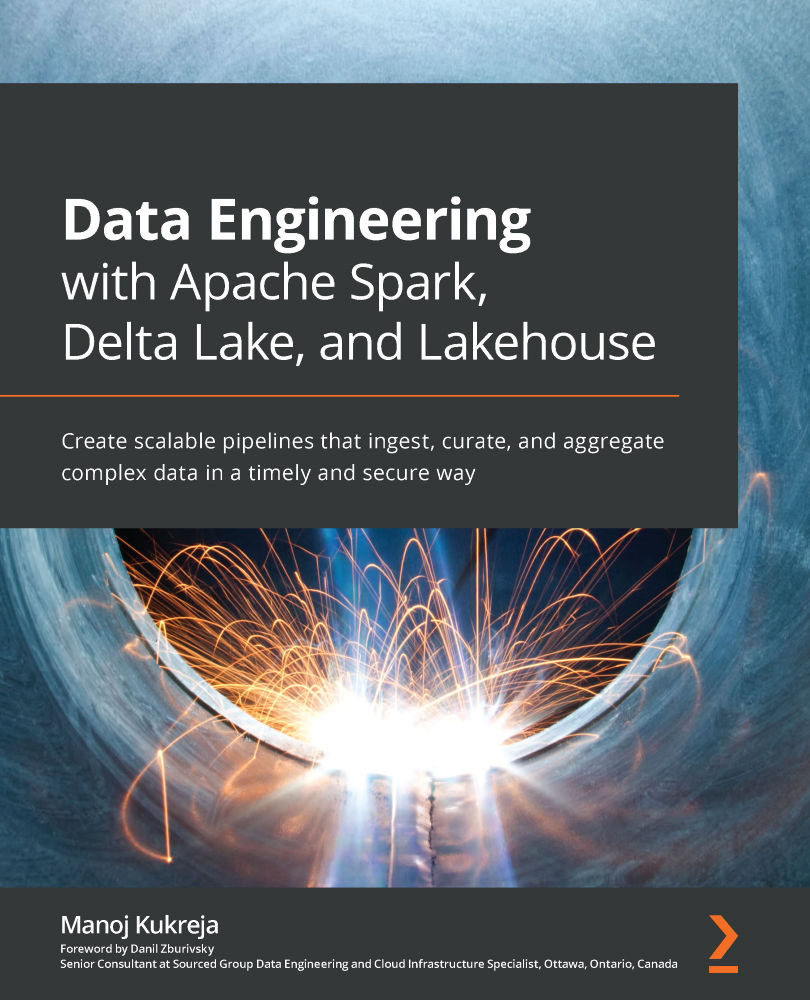
Data Engineering with Apache Spark, Delta Lake, and Lakehouse
€36.99
Snowflake Cookbook
€37.99
Total 113.97 Stars icon
Banner background image

Table of Contents

11 Chapters
Chapter 1: Getting Started with Snowflake Chevron down icon Chevron up icon
Chapter 2: Managing the Data Life Cycle Chevron down icon Chevron up icon
Chapter 3: Loading and Extracting Data into and out of Snowflake Chevron down icon Chevron up icon
Chapter 4: Building Data Pipelines in Snowflake Chevron down icon Chevron up icon
Chapter 5: Data Protection and Security in Snowflake Chevron down icon Chevron up icon
Chapter 6: Performance and Cost Optimization Chevron down icon Chevron up icon
Chapter 7: Secure Data Sharing Chevron down icon Chevron up icon
Chapter 8: Back to the Future with Time Travel Chevron down icon Chevron up icon
Chapter 9: Advanced SQL Techniques Chevron down icon Chevron up icon
Chapter 10: Extending Snowflake Capabilities Chevron down icon Chevron up icon
Other Books You May Enjoy Chevron down icon Chevron up icon

Customer reviews

Top Reviews
Rating distribution
Full star icon Full star icon Full star icon Full star icon Half star icon 4.2
(17 Ratings)
5 star 58.8%
4 star 23.5%
3 star 0%
2 star 17.6%
1 star 0%
Filter icon Filter
Top Reviews

Filter reviews by


Gary Mersy May 28, 2024
Full star icon Full star icon Full star icon Full star icon Full star icon 5
Very good introduction to data modeling and snowflake modeling.
Feefo Verified review Feefo
Nandkishor Aher Apr 10, 2021
Full star icon Full star icon Full star icon Full star icon Full star icon 5
I am amazed to go through this book. Authors has put their experience in simple yet detailed words that the concepts are easier to understand. I must say, I like the simplicity, to point guidance. I can sense the depth knowledge and have listed small small important aspects very neatly. This book is really a bible one can follow. I am happy with this..hope other would like to experience this too. I congratulate author and Publication team a huge success.
Amazon Verified review Amazon
Tea Anemone Apr 10, 2021
Full star icon Full star icon Full star icon Full star icon Full star icon 5
Snowflake is gaining popularity and no wonder I was excited to get a hold of this book as an introduction to Snowflake’s capabilities. Overall, it provides a good overview of Snowflake functionality, covering a wide range of topics - from basic setup of a Snowflake instance (for free with trial!), data lifecycle management, security, cost management (important topic not to be overlooked in enterprise environment), all the way to advanced tasks such as integrating your Snowflake data warehouse with the rest of your data processing platform.This cookbook is a good find for anyone who wants to educate themselves in basic data warehousing principles: the recipes illustrate day to day data engineering tasks. It is interesting to go over the recipe and compare the functionality of a Snowflake instance with, for example, an Azure Synapse SQL pool instance. I guarantee you'll learn something new even if you were in data engineering field for a while.My only disappointment was that all recipes pertaining to external data storage refer to AWS. If you use a different platform (Snowflake supports Azure and Google Cloud as well) - prepare to invest additional time into figuring out how to setup and connect to those sources, because those specifics are completely omitted from the recipes.
Amazon Verified review Amazon
Martin Apr 27, 2021
Full star icon Full star icon Full star icon Full star icon Full star icon 5
Ive been using snowflake for a year and I wish I’d had this book from day 1.Cookbooks are as good as the recipes and this one gets you up and running really quickly.How much it will be as reference is open to debate once you get up to speed, I’ll maybe add to the review later, but for those new to Snowflake it does clearly give you details on things that are maybe not that obvious in Snowflake help.One thing I found, following the practical steps you may often be last asking the question “Why?”As it isn’t always clear at the time. But the “How it works sections” afterwards clears thing up in straightforward fashion.I really liked this book, it’s well written and would recommend to help get you started on some pretty cool stuff.
Amazon Verified review Amazon
Dwight Gunning Apr 11, 2021
Full star icon Full star icon Full star icon Full star icon Full star icon 5
I am not an expert in Snowflake, but I am a mid-career data scientist/engineer who needs to keep current with popular and emerging technologies. So, this book turns out to be a great bookshelf read I can skim at a high level or drop into actually coding using the examples in the book. I am also a contractor so having this Snowflake book for when I need it adds to my value. But it’s not just for experts or mid career people - the Getting Started chapter is easy to read and work through as a beginner. The code examples aren’t too complicated, there are numbered steps and pictures to guide you through the examples. There is also a companion Github repo with examples. So if you are getting started in data engineering and will be working in Snowflake I recommend this book.For people who are already working in Snowflake and consider themselves experts then this Snowflake book might be too easy of high level. But it is great if you want to get productive fast.Overall the book is well written and easy to read, and the hands on examples will get you going in Snowflake. So I recommend this book.
Amazon Verified review Amazon
Get free access to Packt library with over 7500+ books and video courses for 7 days!
Start Free Trial

FAQs

What is the delivery time and cost of print book? Chevron down icon Chevron up icon

Shipping Details

USA:

'

Economy: Delivery to most addresses in the US within 10-15 business days

Premium: Trackable Delivery to most addresses in the US within 3-8 business days

UK:

Economy: Delivery to most addresses in the U.K. within 7-9 business days.
Shipments are not trackable

Premium: Trackable delivery to most addresses in the U.K. within 3-4 business days!
Add one extra business day for deliveries to Northern Ireland and Scottish Highlands and islands

EU:

Premium: Trackable delivery to most EU destinations within 4-9 business days.

Australia:

Economy: Can deliver to P. O. Boxes and private residences.
Trackable service with delivery to addresses in Australia only.
Delivery time ranges from 7-9 business days for VIC and 8-10 business days for Interstate metro
Delivery time is up to 15 business days for remote areas of WA, NT & QLD.

Premium: Delivery to addresses in Australia only
Trackable delivery to most P. O. Boxes and private residences in Australia within 4-5 days based on the distance to a destination following dispatch.

India:

Premium: Delivery to most Indian addresses within 5-6 business days

Rest of the World:

Premium: Countries in the American continent: Trackable delivery to most countries within 4-7 business days

Asia:

Premium: Delivery to most Asian addresses within 5-9 business days

Disclaimer:
All orders received before 5 PM U.K time would start printing from the next business day. So the estimated delivery times start from the next day as well. Orders received after 5 PM U.K time (in our internal systems) on a business day or anytime on the weekend will begin printing the second to next business day. For example, an order placed at 11 AM today will begin printing tomorrow, whereas an order placed at 9 PM tonight will begin printing the day after tomorrow.


Unfortunately, due to several restrictions, we are unable to ship to the following countries:

  1. Afghanistan
  2. American Samoa
  3. Belarus
  4. Brunei Darussalam
  5. Central African Republic
  6. The Democratic Republic of Congo
  7. Eritrea
  8. Guinea-bissau
  9. Iran
  10. Lebanon
  11. Libiya Arab Jamahriya
  12. Somalia
  13. Sudan
  14. Russian Federation
  15. Syrian Arab Republic
  16. Ukraine
  17. Venezuela
What is custom duty/charge? Chevron down icon Chevron up icon

Customs duty are charges levied on goods when they cross international borders. It is a tax that is imposed on imported goods. These duties are charged by special authorities and bodies created by local governments and are meant to protect local industries, economies, and businesses.

Do I have to pay customs charges for the print book order? Chevron down icon Chevron up icon

The orders shipped to the countries that are listed under EU27 will not bear custom charges. They are paid by Packt as part of the order.

List of EU27 countries: www.gov.uk/eu-eea:

A custom duty or localized taxes may be applicable on the shipment and would be charged by the recipient country outside of the EU27 which should be paid by the customer and these duties are not included in the shipping charges been charged on the order.

How do I know my custom duty charges? Chevron down icon Chevron up icon

The amount of duty payable varies greatly depending on the imported goods, the country of origin and several other factors like the total invoice amount or dimensions like weight, and other such criteria applicable in your country.

For example:

  • If you live in Mexico, and the declared value of your ordered items is over $ 50, for you to receive a package, you will have to pay additional import tax of 19% which will be $ 9.50 to the courier service.
  • Whereas if you live in Turkey, and the declared value of your ordered items is over € 22, for you to receive a package, you will have to pay additional import tax of 18% which will be € 3.96 to the courier service.
How can I cancel my order? Chevron down icon Chevron up icon

Cancellation Policy for Published Printed Books:

You can cancel any order within 1 hour of placing the order. Simply contact customercare@packt.com with your order details or payment transaction id. If your order has already started the shipment process, we will do our best to stop it. However, if it is already on the way to you then when you receive it, you can contact us at customercare@packt.com using the returns and refund process.

Please understand that Packt Publishing cannot provide refunds or cancel any order except for the cases described in our Return Policy (i.e. Packt Publishing agrees to replace your printed book because it arrives damaged or material defect in book), Packt Publishing will not accept returns.

What is your returns and refunds policy? Chevron down icon Chevron up icon

Return Policy:

We want you to be happy with your purchase from Packtpub.com. We will not hassle you with returning print books to us. If the print book you receive from us is incorrect, damaged, doesn't work or is unacceptably late, please contact Customer Relations Team on customercare@packt.com with the order number and issue details as explained below:

  1. If you ordered (eBook, Video or Print Book) incorrectly or accidentally, please contact Customer Relations Team on customercare@packt.com within one hour of placing the order and we will replace/refund you the item cost.
  2. Sadly, if your eBook or Video file is faulty or a fault occurs during the eBook or Video being made available to you, i.e. during download then you should contact Customer Relations Team within 14 days of purchase on customercare@packt.com who will be able to resolve this issue for you.
  3. You will have a choice of replacement or refund of the problem items.(damaged, defective or incorrect)
  4. Once Customer Care Team confirms that you will be refunded, you should receive the refund within 10 to 12 working days.
  5. If you are only requesting a refund of one book from a multiple order, then we will refund you the appropriate single item.
  6. Where the items were shipped under a free shipping offer, there will be no shipping costs to refund.

On the off chance your printed book arrives damaged, with book material defect, contact our Customer Relation Team on customercare@packt.com within 14 days of receipt of the book with appropriate evidence of damage and we will work with you to secure a replacement copy, if necessary. Please note that each printed book you order from us is individually made by Packt's professional book-printing partner which is on a print-on-demand basis.

What tax is charged? Chevron down icon Chevron up icon

Currently, no tax is charged on the purchase of any print book (subject to change based on the laws and regulations). A localized VAT fee is charged only to our European and UK customers on eBooks, Video and subscriptions that they buy. GST is charged to Indian customers for eBooks and video purchases.

What payment methods can I use? Chevron down icon Chevron up icon

You can pay with the following card types:

  1. Visa Debit
  2. Visa Credit
  3. MasterCard
  4. PayPal
What is the delivery time and cost of print books? Chevron down icon Chevron up icon

Shipping Details

USA:

'

Economy: Delivery to most addresses in the US within 10-15 business days

Premium: Trackable Delivery to most addresses in the US within 3-8 business days

UK:

Economy: Delivery to most addresses in the U.K. within 7-9 business days.
Shipments are not trackable

Premium: Trackable delivery to most addresses in the U.K. within 3-4 business days!
Add one extra business day for deliveries to Northern Ireland and Scottish Highlands and islands

EU:

Premium: Trackable delivery to most EU destinations within 4-9 business days.

Australia:

Economy: Can deliver to P. O. Boxes and private residences.
Trackable service with delivery to addresses in Australia only.
Delivery time ranges from 7-9 business days for VIC and 8-10 business days for Interstate metro
Delivery time is up to 15 business days for remote areas of WA, NT & QLD.

Premium: Delivery to addresses in Australia only
Trackable delivery to most P. O. Boxes and private residences in Australia within 4-5 days based on the distance to a destination following dispatch.

India:

Premium: Delivery to most Indian addresses within 5-6 business days

Rest of the World:

Premium: Countries in the American continent: Trackable delivery to most countries within 4-7 business days

Asia:

Premium: Delivery to most Asian addresses within 5-9 business days

Disclaimer:
All orders received before 5 PM U.K time would start printing from the next business day. So the estimated delivery times start from the next day as well. Orders received after 5 PM U.K time (in our internal systems) on a business day or anytime on the weekend will begin printing the second to next business day. For example, an order placed at 11 AM today will begin printing tomorrow, whereas an order placed at 9 PM tonight will begin printing the day after tomorrow.


Unfortunately, due to several restrictions, we are unable to ship to the following countries:

  1. Afghanistan
  2. American Samoa
  3. Belarus
  4. Brunei Darussalam
  5. Central African Republic
  6. The Democratic Republic of Congo
  7. Eritrea
  8. Guinea-bissau
  9. Iran
  10. Lebanon
  11. Libiya Arab Jamahriya
  12. Somalia
  13. Sudan
  14. Russian Federation
  15. Syrian Arab Republic
  16. Ukraine
  17. Venezuela