Model parallelism

Model parallelism allows you to distribute the memory and compute requirements of LLMs across multiple GPUs. This enables the training and inference of models too large to fit on a single device, while also improving performance in terms of throughput (tokens per second).

There are three main approaches to model parallelism, each involving splitting the model weights and computation in different ways: data parallelism, pipeline parallelism, and tensor parallelism.

Although these approaches were originally developed for training, we can reuse them for inference by focusing on the forward pass only.

Data parallelism

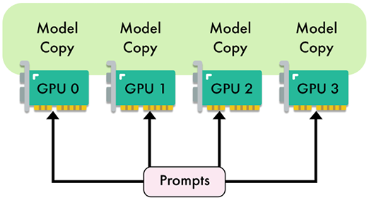
Data parallelism (DP) is the simplest type of model parallelism. It involves making copies of the model and distributing these replicas across different GPUs (see Figure 8.4). Each GPU processes a subset of the data simultaneously. During training, the gradients calculated on each GPU are averaged and used to update the model parameters, ensuring that each replica remains synchronized. This approach is particularly beneficial when the batch size is too large to fit into a single machine or when aiming to speed up the training process.

Figure 8.4 – Illustration of data parallelism with four GPUs

During inference, DP can be useful for processing concurrent requests. By distributing the workload across multiple GPUs, this approach helps reduce latency, as multiple requests can be handled simultaneously. This concurrent processing also increases throughput, since a higher number of requests can be processed at the same time.

However, the effectiveness of DP is limited by the model size and the communication overhead between GPUs. Indeed, replicating the model’s parameters on each GPU is inefficient. This means that this technique only works when the model is small enough to fit into a single GPU, leaving less room for input data and thus limiting the batch size. For larger models or when memory is a constraint, this can be a significant drawback.

Typically, DP is mainly used for training, while pipeline and tensor parallelism are preferred for inference.

Pipeline parallelism

Introduced by Huang et al. in the GPipe paper (2019), pipeline parallelism (PP) is a strategy for distributing the computational load of training and running large neural networks across multiple GPUs.

Unlike traditional DP, which replicates the entire model on each GPU, pipeline parallelism partitions the model’s layers across different GPUs. This approach allows each GPU to handle a specific portion of the model, thereby reducing the memory burden on individual GPUs.

Figure 8.5 – Illustration of pipeline parallelism with four GPUs

As shown in Figure 8.5, in a typical four-way pipeline parallel split, the model is divided into four segments, with each segment assigned to a different GPU. The first 25% of the model’s layers might be processed by GPU 1, the next 25% by GPU 2, and so on. During the forward pass, activations are computed and then passed along to the next GPU. For training, the backward pass follows a similar sequence in reverse, with gradients being propagated back through the GPUs. The number of GPUs is often referred to as the degree of parallelism.

The primary advantage of pipeline parallelism is its ability to significantly reduce the memory requirements per GPU. However, this approach introduces new challenges, particularly related to the sequential nature of the pipeline. One of the main issues is the occurrence of “pipeline bubbles.” These bubbles arise when some GPUs are idle, waiting for activations from preceding layers. This idle time can reduce the overall efficiency of the process.

Micro-batching was developed to mitigate the impact of pipeline bubbles. By splitting the input batch into smaller sub-batches, micro-batching ensures that GPUs remain busier, as the next sub-batch can begin processing before the previous one is fully completed.

Figure 8.6 – Illustration of pipeline parallelism with micro-batching.

Figure 8.6 shows an example of pipeline parallelism with micro-batching. In this example, the pipeline has four stages (F0, F1, F2, F3), and the input batch is divided into four micro-batches. GPU 0 will process forward paths F0,0, F0,1, F0,2, and F0,3, sequentially. Once F0,0 is complete, GPU 1 can immediately start processing F1,0 and so on. After completing these forward passes, GPU 0 waits for the other GPUs to finish their respective forward computations before starting the backward paths (B0,3, B0,2, B0,1, and B0,0).

Pipeline parallelism is implemented in distributed training frameworks like Megatron-LM, DeepSpeed (ZeRO), and PyTorch through the dedicated Pipeline Parallelism for PyTorch (PiPPy) library. At the time of writing, only certain inference frameworks like TensorRT-LLM support pipeline parallelism.

Tensor parallelism

Introduced by Shoeby, Patwary, Puri et al. in the Megatron-LM paper (2019), tensor parallelism (TP) is another popular technique to distribute the computation of LLM layers across multiple devices. In contrast to pipeline parallelism, TP splits the weight matrices found in individual layers. This enables simultaneous computations, significantly reducing memory bottlenecks and increasing processing speed.

In TP, large matrices, such as the weight matrices in MLPs or the attention heads in self-attention layers, are partitioned across several GPUs. Each GPU holds a portion of these matrices and performs computations on its respective slice.

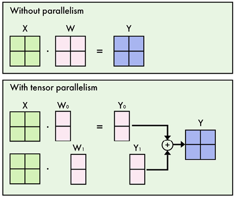
Figure 8.7 – Illustration of column-wise tensor parallelism in an MLP layer (W)

For instance, in an MLP layer, the weight matrix is divided so that each GPU processes only a subset of the weights (see Figure 8.7). The inputs are broadcast to all GPUs, which then independently compute their respective outputs. The partial results are then aggregated through an all-reduce operation, combining them to form the final output.

In the context of self-attention layers, TP is particularly efficient due to the inherent parallelism of attention heads. Each GPU can compute a subset of these heads independently, allowing the model to process large sequences more effectively. This makes TP more efficient than pipeline parallelism, which requires waiting for the completion of previous layers.

Despite its advantages, TP is not universally applicable to all layers of a neural network. Layers like LayerNorm and Dropout, which have dependencies spanning the entire input, cannot be efficiently partitioned and are typically replicated across devices instead. However, these operations can be split on the sequence dimension of the input instead (sequence parallelism). Different GPUs can compute these layers on different slices of the input sequence, avoiding replication of weights. This technique is limited to a few specific layers, but it can provide additional memory savings, especially for very large input sequence lengths.

Moreover, TP necessitates high-speed interconnects between devices to minimize communication overhead, making it impractical to implement across nodes with insufficient interconnect bandwidth.

TP is also implemented in distributed training frameworks like Megatron-LM, DeepSpeed (ZeRO), and PyTorch (FSDP). It is available in most inference frameworks, like TGI, vLLM, and TensorRT-LLM.

Combining approaches

Data, tensor, and pipeline parallelisms are orthogonal techniques that can be combined. Figure 8.8 illustrates how a given model can be split according to each approach:

Figure 8.8 – Illustration of the different model parallelism techniques

Combining these techniques can mitigate their respective issues. Pipeline parallelism provides the greatest memory reduction but sacrifices efficiency, due to pipeline bubbles. This may be ideal if the primary constraint fits the model in the GPU memory. In contrast, if low latency is paramount, then prioritizing tensor parallelism and accepting a larger memory footprint may be the better trade-off. In practice, a model may be split depth-wise into a few pipeline stages, with tensor parallelism used within each stage.

Balancing these tradeoffs and mapping a given model architecture onto available hardware accelerators is a key challenge in deploying LLMs.