Search icon CANCEL
Arrow left icon
Explore Products
Best Sellers
New Releases
Books
Videos
Audiobooks
Learning Hub
Conferences
Free Learning
Arrow right icon
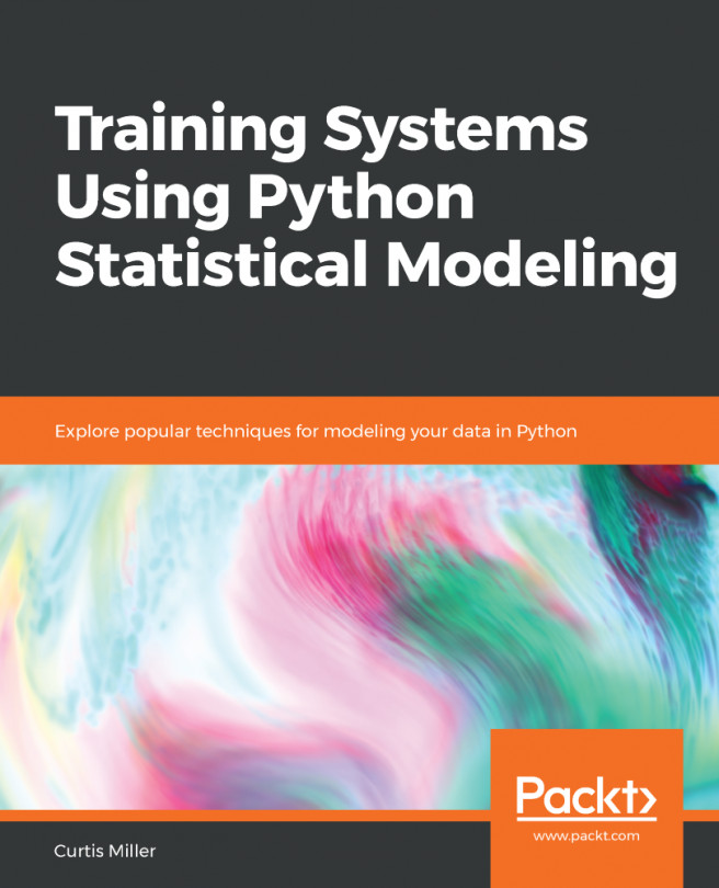
Training Systems Using Python Statistical Modeling

Training Systems Using Python Statistical Modeling: Explore popular techniques for modeling your data in Python

eBook
€15.99 €23.99
Paperback
€29.99
Subscription
Free Trial
Renews at €18.99p/m

What do you get with Print?

Product feature icon Instant access to your digital eBook copy whilst your Print order is Shipped
Product feature icon Paperback book shipped to your preferred address
Product feature icon Download this book in EPUB and PDF formats
Product feature icon Access this title in our online reader with advanced features
Product feature icon DRM FREE - Read whenever, wherever and however you want
Product feature icon AI Assistant (beta) to help accelerate your learning
Table of content icon View table of contents Preview book icon Preview Book

Training Systems Using Python Statistical Modeling

Classical Statistical Analysis

Welcome to the first chapter of our book! In this book, we will use our knowledge of Python and machine learning to create data models and perform statistical analysis on different data schemas. We will learn about various techniques pertaining to statistical learning and how to apply them in data analysis. By the end of this book, you will be confident in using various machine learning models, training them, and learning how to evaluate model results and implement various dimensionality reduction techniques. So, without further ado, let's dive right in! In this chapter, we will look at the following topics:

  • Computing descriptive statistics
  • Classical inference for proportions
  • Classical inference for means
  • Diving into Bayesian analysis
  • Bayesian analysis for proportions
  • Bayesian analysis for means
  • Finding correlations

Technical requirements

The following is required to get the most out of this book:

  • A Windows or Linux system with internet access
  • A basic understanding of Python
  • A basic understanding of the various libraries in Python, such as NumPy, pandas, and matplotlib
  • A basic understanding of Anaconda and Jupyter Notebook

Before starting on this book, the first thing you need to do is to install Anaconda on your system, if you haven't done so already. The installation process is pretty straightforward, as shown in the following steps:

  1. Go to the Anaconda website at https://www.anaconda.com/distribution/#download-section. You will be greeted by the following download section:
  1. Here, you need to select the appropriate installer for your system and download it. Once the download is done, the installation wizard should take you through the whole process easily.
  2. Once the installation is completed, to access the Jupyter Notebook, you should open the Anaconda command line or Terminal and enter the following command:
jupyter notebook

This results in the following screen:

You are now ready to start working!

Computing descriptive statistics

In this section, we will review methods for obtaining descriptive statistics from data that is stored in a pandas DataFrame. We will use the pandas library to compute statistics from the data. So, let's jump right in!

DataFrames come equipped with many methods for computing common descriptive statistics for the data they contain. This is one of the advantages of storing data in DataFrames—working with data stored this way is easy. Getting common descriptive statistics, such as the mean, the median, the standard deviation, and more, is easy for data that is present in DataFrames. There are methods that can be called in order to quickly compute each of these. We will review several of these methods now.

If you want a basic set of descriptive statistics, just to get a sense of the contents of the DataFrame, consider using the describe() method. It includes the mean, standard deviation, an account of how much data there is, and the five-number summary built in.

Sometimes, the statistic that you want isn't a built-in DataFrame method. In this case, you will write a function that works for a pandas series, and then apply that function to each column using the apply() method.

Preprocessing the data

Now let's open up the Jupyter Notebook and get started on our first program, using the methods that we discussed in the previous section:

  1. The first thing we need to do is load the various libraries that we need. We will also load the iris dataset from the scikit-learn library, using the following code:

  1. After importing all the required libraries and the dataset, we will go ahead and create an object called iris_obj, which loads the iris dataset into an object. Then, we will go ahead and use the data method to preview the dataset; and this results in the following output:

Notice that it's a NumPy array. This contains a lot of the data that we want, and each of these columns corresponds to a feature.

  1. We will now see what those feature names are in the following output:

As you can see here, the first column shows the sepal length, the next column shows the sepal width, the third column shows the petal length, and the final column shows the petal width.

  1. Now, there is a fifth column that is not displayed hereit's referred to as the target column. This is stored in a separate array; we will now look at this column as follows:

This displays the target column in an array.

  1. Now, if you want to see the labels of the array header, we can use the following code:

As you can see, the target column consists of data with three different labels. The flowers come from either the setosa, the versicolor, or the virginica species.

  1. Our next step is to take this dataset and turn it into a pandas DataFrame, using the following code:

This results in the following output:

As you can see, we have successfully loaded the data into a DataFrame.

  1. We can see that the species column still shows the various species using numeric values. So, we will replace the final column, which indicates the various species, with strings that indicate the values, rather than numbers, using the following code block:

The following screenshot shows the result:

As you can see, the species column now has the actual species namesthis makes it much easier to work with the data.

Now, for this dataset, the fact that each flower comes from a different species suggests that we may want to actually group the data when we're doing statistical summariestherefore, we can try grouping by species.

  1. So, we will now group the dataset values using the species column as the anchor, and then print out the details of each group to make sure that everything is working. We will use the following lines of code to do so:

This results in the following output:

Now that the data has been loaded and set up, we will use it to perform some basic statistical operations in the next section.

Computing basic statistics

Now we can use the DataFrame that we created to get some basic numbers; we will use the following steps to do so:

  1. We can count how much data there is through the count() method, as shown in the following screenshot:

We can see that there are 150 observations. Note that this excludes NA values (that is, missing values), so it is possible that not all of these observations will be 150.

  1. We can also compute the sample mean, which is the arithmetic average of all the numbers in the dataset, by simply calling the mean() method, as shown in the following screenshot:

Here, we can see the arithmetic means for the numeric columns. The sample mean can also be calculated arithmetically, using the following formula:

  1. Next, we can compute the sample median using the median() method:

Here, we can see the median values; the sample median is the middle data point, which we get after ordering the dataset. It can be computed arithmetically by using the following formula:

Here, x(n) represents ordered data.

  1. We can compute the variance as follows:

The sample variance is a measure of dispersion and is roughly the average squared distance of a data point from the mean. It can be calculated arithmetically, as follows:

  1. The most interesting quantity is the sample standard deviation, which is the square root of the variance. It is computed as follows:

The standard deviation is the square root of the variance and is interpreted as the average distance that a data point is from the mean. It can be represented arithmetically, as follows:

  1. We can also compute percentiles; we do that by defining the value of the percentile that you want to see using the following command:
iris.quantile(.p)

So, here, roughly p% of the data is less than that percentile.

  1. Let's find out the 1st, 3rd, 10th, and 95th percentiles as an example, as follows:
  1. Now, we will compute the interquartile range (IQR) between the 3rd and 1st quantile using the following function:
  1. Other interesting quantities include the maximum value of the dataset, and the minimum value of the dataset. Both of these values can be computed as follows:

Most of the methods mentioned here also work with grouped data. As an exercise, try summarizing the data that we grouped in the previous section, using the previous methods.

  1. Another useful method includes the describe() method. This method can be useful if all you want is just a basic statistical summary of the dataset:

Note that this method includes the count, mean, standard deviations, the five-number summaryfrom the minimum to the maximum, and the quantiles in between. This will also work for grouped data. As an exercise, why don't you try finding the summary of the grouped data?

  1. Now, if we want a custom numerical summary, then we can write a function that will work for a pandas series, and then apply that to the columns of a DataFrame. For example, there isn't a function that computes the range of a dataset, which is the difference between the maximum and the minimum of the dataset. So, we will define a function that can compute the range if it were given a pandas series; here, you can see that by sending it to apply(), you get the ranges that you want:

Notice that I was more selective in choosing columns in terms of which columns to work with. Previously, a lot of the methods were able to weed out columns that weren't numeric; however, to use apply(), you need to specifically select the columns that are numeric, otherwise, you may end up with an error.

  1. We can't directly use the preceding code if we want to filter for grouped data. Instead, we can use the .aggregate() method, as follows:

Thus, we have learned all about computing various statistics using the methods present in pandas. In the next section, we will look at classical statistical inference, specifically with inference for a population proportion.

Classical inference for proportions

In classical statistical inference, we often answer questions about a population, which is a hypothetical group of all possible values and data (including future ones). A sample, on the other hand, is a subset of the population that we use to observe values. In classical statistical inference, we often seek to answer questions about a fixed, non-random, unknown population parameter.

Confidence intervals are computed from data, and are expected to contain θ. We may refer to, say, a 95% confidence intervalthat is, an interval that we are 95% confident contains θ, in the sense that there is a 95% chance that when we compute such an interval, we capture θ in it.

This section focuses on binary variables, where the variable is either a success or a failure, and successes occur with a proportion or probability of p.

An example situation of this is tracking whether a visitor to a website clicked on an ad during their visit. Often, these variables are encoded numerically, with 1 for success, and 0 for a failure.

In classical statistics, we assume that our data is a random sample drawn from a population with a fixed, yet unknown, proportion, p. We can construct a confidence interval based on the sample proportion, which gives us an idea of the proportion of the population. A 95% confidence interval captures the proportion of the population approximately 95% of the time. We can construct confidence intervals using the proportion_confint() function, which is found in the statsmodel package, which allows the easy computation of confidence intervals. Let's now see this in action!

Computing confidence intervals for proportions

The sample proportion is computed by counting the number of successes and dividing this by the total sample size. This can be better explained using the following formula:

Here, N is the sample size and M is the number of success variables; this gives you the sample proportion of successes.

Now, we want to be able to make a statement about the population proportion, which is a fixed, yet unknown, quantity. We will construct a confidence interval for this proportion, using the following formula:

Here, zp is the 100 × pth percentile of the normal distribution.

Now, let's suppose that, on a certain website, out of 1,126 visitors, 310 clicked on a certain ad. Let's construct a confidence interval for the population proportion of visitors who clicked on the ad. This will allow us to predict future clicks. We will use the following steps to do so:

  1. Let's first load the data in the statsmodels package and actually compute the sample proportion, which, in this case, is 310 out of 1,126:

You can see that appropriately 28% of the visitors to the website clicked on the ad on that day.

  1. Our next step is to actually construct a confidence interval using the proportion_confint() function. We assign the number of successes in the count variable, the number of trials in the nobs variable, and the confidence in the alpha variable, as shown in the following code snippet:

As you can see here, with 95% confidence, the proportion is between approximately 25% and 30%.

  1. If we wanted a larger confidence interval, that is, a 99% confidence interval, then we could specify a different alpha, as follows:

Hypothesis testing for proportions

With hypothesis testing, we attempt to decide between two competing hypotheses that are statements about the value of the population proportion. These hypotheses are referred to as the null or alternative hypotheses; this idea is better illustrated in the following diagram:

If the sample is unlikely to be seen at the null hypothesis for true, then we reject the null hypothesis and assume that the alternative hypothesis must be true. We measure how unlikely a sample is by computing a p value, using a test statistic. p values represent the probability of observing a test statistic that is, at least, as contradictory to the null hypothesis as the one computed. Small p values indicate stronger evidence against the null hypothesis. Statisticians often introduce a cutoff and say that if the p value is less than, say, 0.05, then we should reject the null hypothesis in favor of the alternative. We can choose any cutoff we want, depending on how strong we want the evidence against the null hypothesis to be before rejecting it. I don't recommend making your cutoff greater than 0.05. So, let's examine this in action.

Let's say that the website's administrator claims that 30% of visitors to the website clicked on the advertisement—is this true? Well, the sample proportion will never exactly match this number, but we can still decide whether the sample proportion is evidence against this number. So, we're going to test the null hypothesis that p = 0.3, which is what the website administrator claims, against the alternative hypothesis that p0.3. So, now let's go ahead and compute the p value.

First, we're going to import the proportions_ztest() function. We give it how many successes there were in the data, the total number of observations, the value of p under the null hypothesis, and, additionally, we tell it what type of alternative hypothesis we're using:

We can see the result here; the first value is the test statistic and the second one is the p value. In this case, the p value is 0.0636, which is greater than 0.05. Since this is greater than our cutoff, we conclude that there is not enough statistical evidence to disagree with the website administrator.

Testing for common proportions

Now, let's move on to comparing the proportions between two samples. We want to know whether the samples were drawn from populations with the same proportion or not. This could show up in the context, such as A/B testing, where a website wants to determine which of two types of ads generates more clicks.

We can still use the statsmodels function, proportions_ztest(), but we now pass NumPy arrays to the count and nobs arguments, which contain the relevant data for the two samples.

So, our website wants to conduct an experiment. The website will show some of its visitors different versions of an advertisement created by a sponsor. Users are randomly assigned by the server to either Version A or Version B. The website will track how often Version A was clicked on and how often Version B was clicked on by its users. On a particular day, 516 visitors saw Version A and 510 saw Version B. 108 of those who saw Version A clicked on it, and 144 who saw Version B clicked on it. So, we want to know which ad generated more clicks.

We're going to be testing the following hypotheses:

Let's go ahead and import the numpy library. When we import NumPy, we're going to use NumPy arrays to contain our data, as follows:

We will then assign the arrays and define the alternative as two-sided, as follows:

We end up with a p value of around 0.0066, which is small in our case, so we reject the null hypothesis. It appears that the two ads do not have the same proportion of clicks. We have looked at hypothesis testing for proportions. We will now look at applying everything that we have learned to mean values.

Classical inference for means

We'll continue along a similar line to the previous section, in discussing classical statistical methods, but now in a new context. This section focuses on the mean of data that is quantitative, and not necessarily binary. We will demonstrate how to construct confidence intervals for the population mean, as well as several statistical tests that we can perform. Bear in mind throughout this section that we want to infer from a sample mean properties about a theoretical, unseen, yet fixed, population mean. We also want to compare the means of multiple populations, so as to determine whether they are the same or not.

When we assume that the population is a normal distribution, otherwise known as a classic bell curve, then we may use confidence intervals constructed using the t-distribution. These confidence intervals assume a normal distribution but tend to work well for large sample sizes even if the data is not normally distributed. In other words, these intervals tend to be robust. Unfortunately, statsmodels does not have a stable function with an easy user interface for competing these confidence intervals; however, there is a function, called _tconfint_generic(), that can compute them. You need to supply a lot of what this function needs to compute the confidence interval yourself. This means supplying the sample mean, the standard error of the mean, and the degrees of freedom, as shown in the following diagram:

As this looks like an unstable function, this procedure could change in future versions of statsmodels.

Computing confidence intervals for means

Consider the following scenarioyou are employed by a company that fabricates chips and other electronic components. The company wants you to investigate the resistors that it uses in producing its components. In particular, while the resistors used by the company are labeled with a particular resistance, the company wants to ensure that the manufacturer of the resistors produces high-quality products. In particular, when they label a resistor as having 1,000 Ω, they want to know that resistors of that type do, in fact, have 1,000 Ω, on average:

  1. Let's first import NumPy, and then define our dataset in an array, as follows:
  1. We read in this dataset, and the mean resistance is displayed as follows:

Now, we want to know whether it is close to 0 or not. The following is the formula for the confidence interval:

Here, x is the sample mean, s is the sample distribution, α is one minus the confidence level, and tv,p is the pth percentile of the t-distribution with v degrees of freedom.

  1. We're going to import the _tconfint_generic() function from statsmodels. The following code block contains the statement to import the function:
I don't believe that this function is stable, which means that this code could change in the future.
  1. Our next step is to define all the parameters that we will assign to the function. We are going to assign our mean, standard deviation, degrees of freedom, the confidence limit, and the alternative, which is two-sided. This results in the following output:

You will notice that 1 is not in this confidence interval. This might lead you to suspect that the resistors that the supplier produces are not being properly manufactured.

Hypothesis testing for means

We can test the null hypothesis that the population mean (often denoted by the Greek letter μ) is equal to a hypothesized number (denoted by μ0) against an alternative hypothesis. The alternative will state that the population mean is either less than, greater than, or not equal to the mean we hypothesized. Again, if we assume that data was drawn from a normal distribution, we can use t-proceduresnamely, the t-test. This test works well for non-normal data, when the sample size is large. Unfortunately, there is not a stable function in statmodels for this test; however, we can use the _tstat_generic() function, from version 0.8.0, for this test. We may need to hack it a little bit, but it can get us the p value for this test.

So, the confidence interval that you computed earlier suggests that the resistors this manufacturer is sending your company are not being properly manufactured. In fact, you believe that their resistors have a resistance level that's less than that specified. So, you'll be testing the following hypotheses:

The first hypothesis indicates that the company is telling the truth, so you assumed that at the outset. The alternative hypothesis says that the true mean is less than 1,000 Ω. So, you are going to assume that the resistance is normally distributed, and this will be your test statistic. We will now perform the hypotheses testing using the following steps:

  1. Our first step is to import the _tstat_generic() function, as follows:
  1. Then, we're going to define all the parameters that will be used in the function. This includes the mean of the dataset, the mean under the null hypothesis, the standard deviation, and so on. This results in the following output:

So, we compute the p value, and this p value is minuscule. So, clearly, the resistance of the resistors the manufacturer makes is less than 1,000Ωtherefore, your company is being fleeced by this manufacturer; they're not actually producing quality parts. We can also test whether two populations have the same mean, or whether their means are different in some way.

Testing with two samples

If we assume that our data was drawn from normal distributions, the t-test can be used. For this test, we can use the statsmodels function, ttest_ind(). This is a more stable function from the package, and uses a different interface. So, here, we're going to test for a common mean.

Let's assume that your company has decided to stop outsourcing resistor production, and they're experimenting with different methods so that they can start producing resistors in-house. So, they have process A and process B, and they want you to test whether the mean resistance for these two processes is the same, or whether they're different. Therefore, you feel safe, assuming again that the resistance level of resistors is normally distributed regardless of whatever manufacturing process is employed, and you don't assume that they have the same standard deviation. Thus, the test statistic is as follows:

So, let's use this test statistic to perform your test:

Our first step is to load in the data, as follows:

Our next step is to load and define the ttest_ind function, as follows:

This will give us a p value. In this case, the p value is 0.659this is a very large p value. It suggests that we should not reject the null hypothesis, and it appears that the two processes produce resistors with the same mean level of resistance.

One-way analysis of variance (ANOVA)

One-way ANOVA tests whether all groups share a common mean with their own sample. The null hypothesis assumes that all populations share the same mean, while the alternative hypothesis simply states that the null hypothesis is false. One-way ANOVA assumes that data was drawn from normal distributions with a common standard deviation. While normality can be relaxed for larger sample sizes, the assumption of common standard deviation is, in practice, more critical.

Before performing this test, let's consider doing a visual check to see whether the data has a common spread. For example, you could create side-by-side box and whisker plots. If the data does not appear to have a common standard deviation, you should not perform this test.

The f_oneway() function from SciPy can perform this test; so, let's start performing one-way ANOVA.

Your company now has multiple processes. Therefore, before you were able to return your report for the other two, you were given data for processes C, D, and E. Your company wants to test whether all of these processes have the same mean level of resistance or whether this is not truein other words, whether one of these processes has a different mean level of resistance. So, let's get into it:

  1. We will first define the data for these other processes, as follows:
  1. We're going to use the f_oneway() function from SciPy to perform this test, and we can simply pass the data from each of these samples to this function, as follows:
  1. This will give us the p value, which, in this case, is 0.03:

This appears to be small, so we're going to reject the null hypothesis that all processes yield resistors with the same level of resistance. It appears at least one of them has a different mean level of resistance.

This concludes our discussion of classical statistical methods for now. We will now move on to discussing Bayesian statistics.

Diving into Bayesian analysis

Welcome to the first section on Bayesian analysis. This section discusses the basic concepts used in Bayesian statistics. This branch of statistics often involves classical statistics and requires more knowledge of mathematics and probability, but it seems to be popular in computer science. This section will get you up to speed with what you need to know to understand and perform Bayesian statistics.

All Bayesian statistics are based on Bayes' theorem; in Bayesian statistics, we consider an event or parameter as a random variable. For example, suppose that we're talking about a parameter; we give a prior distribution to the parameter, and a likelihood of observing a certain outcome given the value of the parameter. Bayes' theorem lets us compute the posterior distribution of the parameter, which we can use to reach conclusions about it. The following formula shows Bayes' theorem:

All Bayesian statistics are an exercise in applying this theorem. The α symbol means proportional to, that is, that the two sides differ by a multiplicative factor.

How Bayesian analysis works

I assume that we are interested in the value of a parameter, such as the mean or proportion. We start by giving this parameter a prior distribution quantifying our beliefs about where the parameter is located, based on what we believe about it before collecting data. There are lots of ways to pick the prior; for example, we could pick an uninformative prior that says little about a parameter's value. Alternatively, we could use a prior that gives beliefs based on, say, previous studies, therefore biasing the value of the parameter to these values.

Then, we collect data and use it to compute the posterior distribution of the parameter, which is our updated belief about its location after seeing new evidence. This posterior distribution is then used to answer all our questions about the parameter's location. Note that the posterior distribution will answer all questions with probabilities. This means that we don't say whether the parameter is in a particular region or not, but the probability that it is located in that region instead. In general, the posterior distribution is difficult to compute. Often, we need to rely on computationally intensive methods such as Monte Carlo simulation to estimate posterior quantities. So, let's examine a very simple example of Bayesian analysis.

Using Bayesian analysis to solve a hit-and-run

In this case, we're going to be solving a hit-and-run. In a certain city, 95% of cabs are owned by the Yellow Cab Company, and 5% are owned by Green Cab, Inc. Recently, a cab was involved in a hit-and-run accident, injuring a pedestrian. A witness saw the accident and claimed that the cab that hit the pedestrian was a green cab. Tests by investigators revealed that, under similar circumstances, this witness is correctly able to identify a green cab 90% of the time and correctly identify a yellow cab 85% of the time. This means that they incorrectly call a yellow cab a green cab 15% of the time, and incorrectly call a green cab a yellow cab 10% of the time. So, the question is, should we pursue Green Cab, Inc.?

The following formula shows Bayes' theorem:

Here, H represents the event that a green cab hit the pedestrian, while G represents the event that the witness claims to have seen a green cab.

So, let's encode these probabilities, as follows:

Now that we have these probabilities, we can use Bayes' theorem to compute the posterior probability, which is given as follows:

So, the result is that the prior probability that the cab was actually green was 0.05, which was very low. The posterior probability, that is, the probability that the cab that hit the pedestrian was green, given that the witness said the cab was green, is now 32%, which is higher than that number, but it is still less than 50%.

Additionally, considering that this city consists only of yellow cabs and green cabs, this indicates that even though the witness saw a green cab or claimed to have seen a green cab, there are too few green cabs and the witness is not accurate enough to override how few green cabs there are. This means that it's still more likely that the pedestrian was hit by a yellow cab and that the witness made a mistake.

Now, let's take a look at some useful applications of Bayesian analysis. We will go through topics similar to those seen previously, but from the Bayesian perspective.

Bayesian analysis for proportions

In this section, we'll revisit inference for proportions, but from a Bayesian perspective. We will look at Bayesian methods for analyzing proportions of success in a group. This includes talking about computing credible intervals, and the Bayesian version of hypothesis testing for both one and two samples.

Conjugate priors are a class of prior probability distributions common in Bayesian statistics. A conjugate prior is a prior distribution such that the posterior distribution belongs to the same family of probability distributions as the prior. For binary data, the beta distribution is a conjugate prior. This is a distribution defined where only values in the (0, 1) interval have a chance of appearing. They are specified by two parameters. In a trial, if there are M successes out of N trials, then the posterior distribution is the prior distribution when we add M to the first parameter of the prior, and N - M to the second parameter of the prior. This concentrates the distribution to the observed population proportion.

Conjugate priors for proportions

So, let's see this in action. For data that takes values of either 0 or 1, we're going to use the beta distribution as our conjugate prior. The notation that is used to refer to the beta distribution is B(α, β).

α - 1 can be interpreted as imaginary prior successes, and β - 1 can be interpreted as imaginary prior failures. That's if you have added the data to your datasetimaginary successes and imaginary failures.

If α = β = 1, then we interpret this as being no prior successes or failures; therefore, every probability of success, θ, is equally likely in some sense. This is referred to as an uninformative prior. Let's now implement this using the following steps:

  1. First, we're going to import the beta function from scipy.stats; this is the beta distribution. In addition to this, we will import the numpy library and the matplotlib library, as follows:
  1. We're then going to plot the function and see how it looks, using the following code:

This results in the following output:

So, if we plot β when α=1 and β=1, we end up with a uniform distribution. In some sense, each p is equally likely.

  1. Now, we will use a=3 and b=3, to indicate two imaginary successes and two imaginary failures, which gives us the following output:

Now, our prior distribution biases our data toward 0.5in other words, it is equally likely to succeed as it is to fail.

Given a sample size of N, if there are M successes, then the posterior distribution when the prior is β, with the parameters (α, β), will be B (α + M, β + N - M). So, let's reconsider an earlier example; we have a website with 1,126 visitors. 310 clicked on an ad purchased by a sponsor, and we want to know what proportion of individuals will click on the ad in general.

  1. So, we're going to use our prior distribution beta (3, 3). This means that the posterior distribution will be given by the beta distribution, with the first parameter, 313, and the second parameter, 819. This is what the prior distribution and posterior distribution looks like when plotted against each other:

The blue represents the prior distribution, and red represents the posterior distribution.

Credible intervals for proportions

Bayesian statistics doesn't use confidence intervals but credible intervals instead. We specify a probability, and that will be the probability that the parameter of interest lies in the credible interval. For example, there's a 95% chance that θ lies in its 95% credible interval. We compute credible intervals by computing the quantiles from the posterior distribution of the parameter, so that the chosen proportion of the posterior distribution lies between these two quantiles.

So, I've already gone ahead and written a function that will compute credible intervals for you. You give this function the number of successes, the total sample size, the first argument of the prior and the second argument of the prior, and the credibility (or chance of containing θ) of the interval. You can see the entire function as follows:

So, here is the function; I've already written it so that it works for you. We can use this function to compute credible intervals for our data.

So, we have a 95% credible interval based on the uninformative prior, as follows:

Therefore, we believe that θ will be between 25% and 30%, with a 95% probability.

The next one is the same interval when we have a different priorthat is, the one that we actually used before and is the one that we plotted:

The data hasn't changed very much, but still, this is going to be our credible interval.

The last one is the credible interval when we increase the level of credibility to .99 or the probability of containing the true parameter:

Since this probability is higher, this must be a longer interval, which is exactly what we see, although it's not that much longer.

Bayesian hypothesis testing for proportions

Unlike classical statistics, where we say a hypothesis is either right or wrong, Bayesian statistics holds that every hypothesis is true, with some probability. We don't reject hypotheses, but simply ignore them if they are unlikely to be true. For one sample, computing the probability of a hypothesis can be done by considering what region of possible values of θ correspond to the hypothesis being true, and using the posterior distribution of θ to compute the probability that θ is in that region.

In this case, we need to use what's known as the cumulative distribution function (CDF) of the posterior distribution. This is the probability that a random variable is less than or equal to a quantity, x. So, what we want is the probability that θ is greater than 0.3 when D is given, that is, if we are testing the website administrator's claim that there are at least 30% of visitors to the site clicking on the ad.

So, we will use the CDF function and evaluate it at 0.3. This is going to correspond to the administrator's claim. This will give us the probability that more than 30% of visitors clicked on the ad. The following screenshot shows how we define the CDF function:

What we end up with is a very small probability, therefore, it's likely that the administrator is incorrect.

Now, while there's a small probability, I would like to point out that this is not the same thing as a p value. A p value says something completely different; a p value should not be interpreted as the probability that the null hypothesis is true, whereas, in this case, this can be interpreted as a probability that the hypothesis we asked is true. This is the probability that data is greater than 0.3, given the data that we saw.

Comparing two proportions

Sometimes, we may want to compare two proportions from two populations. Crucially, we will assume that they are independent of each other. It's difficult to analytically compute the probability that one proportion is less than another, so we often rely on Monte Carlo methods, otherwise known as simulation or random sampling.

We randomly generate the two proportions from their respective posterior distributions, and then track how often one is less than the other. We use the frequency we observed in our simulation to estimate the desired probability.

So, let's see this in action; we have two parameters: θA and θB. These correspond to the proportion of individuals who click on an ad from format A or format B. Users are randomly assigned to one format or the other, and the website tracks how many viewers click on the ad in the different formats.

516 visitors saw format A and 108 of them clicked it. 510 visitors saw format B and 144 of them clicked it. We use the same prior for both θA and θB, which is beta (3, 3). Additionally, the posterior distribution for θA will be B (111, 411) and for θB, it will be B (147, 369). This results in the following output:

We now want to know the probability of θA being less than θBthis is difficult to compute analytically. We can randomly simulate θA and θB, and then use that to estimate this probability. So, let's randomly simulate one θA, as follows:

Then, randomly simulate one θB, as follows:

Finally, we're going to do 1,000 simulations by computing 1,000 θA values and 1,000 θB values, as follows:

This is what we end up with; here, we can see how often θA is less than θB, that is, θA was 996 times less than θB. So, what's the average of this? Well, it is 0.996; this is the probability that θA is less than θB, or an estimate of that probability. Given this, it seems highly likely that more people clicked on the ad for format B than people who clicked on the ad for format A.

That's it for proportions. Next up, we will look at Bayesian methods for analyzing the means of quantitative data.

Bayesian analysis for means

Now we'll move on to discussing Bayesian methods for analyzing the means of quantitative data. This section is similar to the previous one on Bayesian methods for analyzing proportions, but it focuses on the means of quantitative data. Here, we look at constructing credible intervals and performing hypothesis testing.

Suppose that we assume that our data was drawn from a normal distribution with an unknown mean, μ, and an unknown variance, σ2. The conjugate prior, in this case, will be the normal inverse gamma (NIG) distribution. This is a two-dimensional distribution, and gives a posterior distribution for both the unknown mean and the unknown variance.

In this section, we only care about what the unknown mean is. We can get a marginal distribution for the mean from the posterior distribution, which depends only on the mean. The variance no longer appears in the marginal distribution. We can use this distribution for our analysis.

So, we say that the mean and the standard deviation, both of these things being unknown, were drawn from a NIG distribution with the parameters of μ0, μ, α, and β. This can be represented using the following formula:

The posterior distribution after you have collected data can be represented as follows:

In this case, I'm interested in the marginal distribution of the mean, μ, under the posterior distribution. The prior marginal distribution of μ is t(2α), which means that it follows a t-distribution with two alpha degrees of freedom; this is the posterior marginal distribution of the following formula:

Here, it is t(2α + n).

This is all very complicated, so I've written five helper functions, which are as follows:

  • Compute the probability density function (PDF) of (μ,σ2), which is useful for plotting.
  • Compute the parameters of the posterior distribution of (μ,σ2).
  • Compute the PDF and CDF of the marginal distribution of μ (for either the prior or posterior distribution).
  • Compute the inverse CDF of the marginal distribution of μ (for either the prior or posterior distribution).
  • Simulate a draw from the marginal distribution of μ (for either the prior or posterior distribution).

We will apply these functions using the following steps:

  1. So, first, we're going to need these libraries:
  1. Then, the dnig() function computes the density of the normal inverse gamma distributionthis is helpful for plotting, as follows:
  1. The get_posterior_nig() function will get the parameters of the posterior distribution, where x is our data; and these four parameters specify the parameters of the prior distribution, but will be returned as a tuple that contains the parameters of the posterior distribution:
  1. The dnig_mu_marg() function is the density function of the marginal distribution for μ. It will be given a floating-point number that you want to evaluate the PDF on. This will be useful if you want to plot the marginal distribution of μ:
  1. The pnig_mu_marg() function computes the CDF of the marginal distribution; that is, the probability of getting a value less than or equal to your value of x, which you pass to the function. This'll be useful if you want to do things such as hypothesis testing or computing the probability that a hypothesis is true under the posterior distribution:
  1. The qunig_mu_marg() function will be the inverse CDF, however, you give it a probability, and it will give you the quantile associated with that probability. This is a function that's going to be useful if you want to construct, say, credible intervals:
  1. Finally, the rnig_mu_marg() function draws random numbers from the marginal distribution of μ from a normal inverse gamma distribution, so this'll be useful if you want to sample from the posterior distribution of μ:
  1. Now, we will perform a short demonstration of what the dnig() function does, so you can get an idea of what the normal inverse gamma distribution looks like, using the following code:

This results in the following output:

This plot gives you a sense of what the normal inverse gamma looks like. Therefore, most of the density is concentrated in this region, but it starts to spread out.

Credible intervals for means

Getting a credible interval for the mean is the same as the one for proportions, except that we will work with the marginal distribution for just the unknown mean from the posterior distribution.

Let's repeat a context that we used in the Computing confidence intervals for means section of this chapter. You are employed by a company that's fabricating chips and other electronic components. The company wants you to investigate the resistors it's using to produce its components. These resistors are being manufactured by an outside company and they've been specified as having a particular resistance. They want you to ensure that the resistors being produced and sent to them are high quality productsspecifically, that when they are labeled with a resistance level of 1,000 Ω, then they do in fact have a resistance of 1,000 Ω. So, let's get started, using the following steps:

  1. We will use the same dataset as we did in the Computing confidence intervals for means section.
  1. Now, we're going to use the NIG (1, 1, 1/2, 0.0005) distribution for our prior distribution. You can compute the parameters of the posterior distribution using the following code:

When the parameters of the distribution are computed, it results in the following output:

It looks as if the mean has been moved; you now have 105 observations being used as your evidence.

  1. Now, let's visualize the prior and posterior distributionspecifically, their marginal distributions:

Blue represents the prior distribution, and red represents the posterior distribution. It appears that the prior distribution was largely uninformative about where the true resistance was, while the posterior distribution strongly says that the resistance is approximately 0.99.

  1. Now, let's use this to compute a 95% credible interval for the mean of μ. I have written a function that will do this for you, where you feed it data and also the parameters of the prior distribution, and it will give you a credible interval with a specified level of credibility. Let's run this function as follows:
  1. Now, let's compute the credible interval:

Here, what we notice is that 1 is not in this credible interval, so there's a 95% chance that the true resistance level is between 0.9877 and 0.9919.

Bayesian hypothesis testing for means

Hypothesis testing is similar, in principle, to what we have done previously; only now, we are using the marginal distribution of the mean from the posterior distribution. We compute the probability that the mean lies in the region corresponding to the hypothesis being true.

So, now, you want to test whether the true mean is less than 1,000 Ω. To do this, we get the parameters of the posterior distribution, and then feed these to the pnig_mu_marg() function:

We end up with a probability that is almost 1. It is all but certain that the resistors are not properly calibrated.

Testing with two samples

Suppose that we want to compare the means of two populations. We start by assuming that the parameters of the two populations are independent and compute their posterior distributions, including the marginal distributions of the means. Then, we use Monte Carlo methods, similar to those used previously, to estimate the probability that one mean is less than the other. So, let's now take a look at two-sample testing.

Your company has decided that it no longer wants to stick with this manufacturer. They want to start producing resistors in-house, and they're looking at different methods for producing these resistors. Right now, they have two manufacturing processes known as process A and process B, and you want to know whether the mean for process A is less than the mean for process B. So, what we'll do is use Monte Carlo methods, as follows:

  1. Collect data from both processes and compute the posterior distributions for both μA and μB.
  2. Simulate random draws of μA and μB from the posterior distributions.
  3. Compute how often μA is less than μB to estimate the probability that μA > μB.

So, first, let's get the dataset for the two processes:

We get the posterior distributions for both processes as follows:

Now, let's simulate 1,000 draws from the posterior distributions:

Here are the random μA values:

Here are the random μB values:

Here is when μA is less than μB:

Finally, we add these up and take the mean, as follows:

We can see that about 65.8% of the time μA is less than μB. This is higher than 50%, which suggests that μA is probably less than μB, but this is not a very actionable probability. 65.8% is not a probability high enough to strongly suggest a change needs to be made.

So, that's it for Bayesian statistics for now. We will now move on to computing correlations in datasets.

Finding correlations

In the final section of this chapter, we will learn about computing correlations using pandas and SciPy. We will look at how to use pandas and SciPy to compute correlations in datasets, and also explore some statistical tests to detect correlation.

In this section, I have used Pearson's correlation coefficient, which quantifies how strongly two variables are linearly correlated. This is a unitless number that takes values between -1 and 1. The sign of the correlation coefficient indicates the direction of the relationship. A positive r indicates that as one variable increases, the other tends to increase; while a negative r indicates that as one variable increases, the other tends to decrease. The magnitude indicates the strength of the relationship. If r is close to 1 or -1, then the relationship is almost a perfect linear relationship, while an r that is close to 0 indicates no linear relationship. The NumPy corrcoef() function computes the number for two NumPy arrays.

So, here's the correlation coefficient's definition. We're going to work with what's known as the Boston housing price dataset. This is known as a toy dataset, and is often used for evaluating statistical learning methods. I'm only interested in looking at correlations between the variables in this dataset.

Note that we will be using a slightly modified version of the dataset, which can be found in the GitHub repository for this chapter.

We will use the following steps:

  1. We will first load up all the required libraries, as follows:
  1. We will then load in the dataset using the following code:
  1. Then, we will print the dataset information, so that we can have a look at it, as follows:

So, these attributes tell us what this dataset contains. It has a few different variables such as, for example, the crime rate by town, the proportion of residential land zones, non-retail business acres, and others. Therefore, we have a number of different attributes for you to play with.

  1. We will now load the actual dataset, as follows:

This is going to very useful to us. Now, let's take a look at the correlation between the two variables.

  1. We're going to import the corrcoef() function, and we're going to look at one of the columns from this dataset as if it were a NumPy array, as follows:

It started out as a NumPy array, but it's perfectly fine to just grab a pandas series and turn it into an array.

  1. Now we're going to take corrcoef(), and compute the correlation between the crime rate and the price:

We can see that the numbers in the matrix are the same.

The number in the off-diagonal entries corresponds to the correlation between the two variables. Therefore, there is a negative relationship between crime rate and price, which is not surprising. As the crime rate increases, you would expect the price to decrease. But this is not a very strong correlation. We often want correlations not just for two variables, but for many combinations of two variables. We can use the pandas DataFrame corr() method to compute what's known as the correlation matrix. This matrix contains correlations for every combination of variables in our dataset.

  1. So, let's go ahead and compute a correlation matrix for the Boston dataset, using the corr() function:

These are all correlations. Every entry off the diagonal will have a corresponding entry on the other side of the diagonal—this is a symmetric matrix. Now, while this matrix contains all the data that we might want, it is very difficult to read.

  1. So, let's use a package called seaborn, as this is going to allow us to plot a heatmap. A heatmap has colors with differing intensities for how large or small a number tends to be. So, we compute a heatmap and plot it as follows:

The preceding screenshot shows the resulting map. Here, black indicates correlations close to -1, and very light colors indicate correlations that are close to 1. From this heatmap, we can start to see some patterns.

Testing for correlation

SciPy contains the pearsonr() function in its statistics module, which not only computes the correlation between two variables but also allows for hypothesis testing to detect correlation. Rejecting the null hypothesis will signify that the correlation between the two variables, in general, is not 0. However, be aware that rejecting the null hypothesis does not automatically signify a meaningful relationship between the two variables. It's possible that the correlation is not 0, but still too small to be meaningful. This is especially true when performing the test on large samples.

We're going to do a statistical test using the following hypotheses:

We import the pearsonr() function, and we run it on crime and price to see whether these things are correlated with statistical significance:

Here, we have a very small p value, which suggests that yes, indeed, the crime rate and the price of a home appear to be correlated. If we had to take a guess, then we would say that it would be negatively correlated.

Summary

That's all for this chapter on classical statistical methods. We learned about computing descriptive statistics for data and we learned how to implement classical inference for proportions. We also learned how to implement inference for means. We then explored Bayesian analysis and examined how to apply it to analyze proportions and means. Finally, we learned how to find correlations using pandas and SciPy.

In the next chapter, we will learn about some basic machine learning theory.

Left arrow icon Right arrow icon
Download code icon Download Code

Key benefits

  • Get started with Python's rich suite of libraries for statistical modeling
  • Implement regression and clustering, and train neural networks from scratch
  • Discover real-world examples on training end-to-end machine learning systems in Python

Description

Python's ease-of-use and multi-purpose nature has made it one of the most popular tools for data scientists and machine learning developers. Its rich libraries are widely used for data analysis, and more importantly, for building state-of-the-art predictive models. This book is designed to guide you through using these libraries to implement effective statistical models for predictive analytics. You’ll start by delving into classical statistical analysis, where you will learn to compute descriptive statistics using pandas. You will focus on supervised learning, which will help you explore the principles of machine learning and train different machine learning models from scratch. Next, you will work with binary prediction models, such as data classification using k-nearest neighbors, decision trees, and random forests. The book will also cover algorithms for regression analysis, such as ridge and lasso regression, and their implementation in Python. In later chapters, you will learn how neural networks can be trained and deployed for more accurate predictions, and understand which Python libraries can be used to implement them. By the end of this book, you will have the knowledge you need to design, build, and deploy enterprise-grade statistical models for machine learning using Python and its rich ecosystem of libraries for predictive analytics.

Who is this book for?

If you are a data scientist, a statistician or a machine learning developer looking to train and deploy effective machine learning models using popular statistical techniques, then this book is for you. Knowledge of Python programming is required to get the most out of this book.

What you will learn

  • Understand the importance of statistical modeling
  • Learn about the different Python packages for statistical analysis
  • Implement algorithms such as Naive Bayes and random forests
  • Build predictive models from scratch using Python s scikit-learn library
  • Implement regression analysis and clustering
  • Learn how to train a neural network in Python
Estimated delivery fee Deliver to Portugal

Premium delivery 7 - 10 business days

€17.95
(Includes tracking information)

Product Details

Country selected
Publication date, Length, Edition, Language, ISBN-13
Publication date : May 20, 2019
Length: 290 pages
Edition : 1st
Language : English
ISBN-13 : 9781838823733
Category :
Languages :
Tools :

What do you get with Print?

Product feature icon Instant access to your digital eBook copy whilst your Print order is Shipped
Product feature icon Paperback book shipped to your preferred address
Product feature icon Download this book in EPUB and PDF formats
Product feature icon Access this title in our online reader with advanced features
Product feature icon DRM FREE - Read whenever, wherever and however you want
Product feature icon AI Assistant (beta) to help accelerate your learning
Estimated delivery fee Deliver to Portugal

Premium delivery 7 - 10 business days

€17.95
(Includes tracking information)

Product Details

Publication date : May 20, 2019
Length: 290 pages
Edition : 1st
Language : English
ISBN-13 : 9781838823733
Category :
Languages :
Tools :

Packt Subscriptions

See our plans and pricing
Modal Close icon
€18.99 billed monthly
Feature tick icon Unlimited access to Packt's library of 7,000+ practical books and videos
Feature tick icon Constantly refreshed with 50+ new titles a month
Feature tick icon Exclusive Early access to books as they're written
Feature tick icon Solve problems while you work with advanced search and reference features
Feature tick icon Offline reading on the mobile app
Feature tick icon Simple pricing, no contract
€189.99 billed annually
Feature tick icon Unlimited access to Packt's library of 7,000+ practical books and videos
Feature tick icon Constantly refreshed with 50+ new titles a month
Feature tick icon Exclusive Early access to books as they're written
Feature tick icon Solve problems while you work with advanced search and reference features
Feature tick icon Offline reading on the mobile app
Feature tick icon Choose a DRM-free eBook or Video every month to keep
Feature tick icon PLUS own as many other DRM-free eBooks or Videos as you like for just €5 each
Feature tick icon Exclusive print discounts
€264.99 billed in 18 months
Feature tick icon Unlimited access to Packt's library of 7,000+ practical books and videos
Feature tick icon Constantly refreshed with 50+ new titles a month
Feature tick icon Exclusive Early access to books as they're written
Feature tick icon Solve problems while you work with advanced search and reference features
Feature tick icon Offline reading on the mobile app
Feature tick icon Choose a DRM-free eBook or Video every month to keep
Feature tick icon PLUS own as many other DRM-free eBooks or Videos as you like for just €5 each
Feature tick icon Exclusive print discounts

Frequently bought together


Stars icon
Total 84.97
Hands-On Deep Learning Algorithms with Python
€29.99
Hands-On Deep Learning Architectures with Python
€24.99
Training Systems Using Python Statistical Modeling
€29.99
Total 84.97 Stars icon

Table of Contents

8 Chapters
Classical Statistical Analysis Chevron down icon Chevron up icon
Introduction to Supervised Learning Chevron down icon Chevron up icon
Binary Prediction Models Chevron down icon Chevron up icon
Regression Analysis and How to Use It Chevron down icon Chevron up icon
Neural Networks Chevron down icon Chevron up icon
Clustering Techniques Chevron down icon Chevron up icon
Dimensionality Reduction Chevron down icon Chevron up icon
Other Books You May Enjoy Chevron down icon Chevron up icon

Customer reviews

Rating distribution
Full star icon Empty star icon Empty star icon Empty star icon Empty star icon 1
(1 Ratings)
5 star 0%
4 star 0%
3 star 0%
2 star 0%
1 star 100%
Mehdi Dec 18, 2019
Full star icon Empty star icon Empty star icon Empty star icon Empty star icon 1
I expected a deep overview of implementation of statsitcal model, however, it's more like a class project.
Amazon Verified review Amazon
Get free access to Packt library with over 7500+ books and video courses for 7 days!
Start Free Trial

FAQs

What is the delivery time and cost of print book? Chevron down icon Chevron up icon

Shipping Details

USA:

'

Economy: Delivery to most addresses in the US within 10-15 business days

Premium: Trackable Delivery to most addresses in the US within 3-8 business days

UK:

Economy: Delivery to most addresses in the U.K. within 7-9 business days.
Shipments are not trackable

Premium: Trackable delivery to most addresses in the U.K. within 3-4 business days!
Add one extra business day for deliveries to Northern Ireland and Scottish Highlands and islands

EU:

Premium: Trackable delivery to most EU destinations within 4-9 business days.

Australia:

Economy: Can deliver to P. O. Boxes and private residences.
Trackable service with delivery to addresses in Australia only.
Delivery time ranges from 7-9 business days for VIC and 8-10 business days for Interstate metro
Delivery time is up to 15 business days for remote areas of WA, NT & QLD.

Premium: Delivery to addresses in Australia only
Trackable delivery to most P. O. Boxes and private residences in Australia within 4-5 days based on the distance to a destination following dispatch.

India:

Premium: Delivery to most Indian addresses within 5-6 business days

Rest of the World:

Premium: Countries in the American continent: Trackable delivery to most countries within 4-7 business days

Asia:

Premium: Delivery to most Asian addresses within 5-9 business days

Disclaimer:
All orders received before 5 PM U.K time would start printing from the next business day. So the estimated delivery times start from the next day as well. Orders received after 5 PM U.K time (in our internal systems) on a business day or anytime on the weekend will begin printing the second to next business day. For example, an order placed at 11 AM today will begin printing tomorrow, whereas an order placed at 9 PM tonight will begin printing the day after tomorrow.


Unfortunately, due to several restrictions, we are unable to ship to the following countries:

  1. Afghanistan
  2. American Samoa
  3. Belarus
  4. Brunei Darussalam
  5. Central African Republic
  6. The Democratic Republic of Congo
  7. Eritrea
  8. Guinea-bissau
  9. Iran
  10. Lebanon
  11. Libiya Arab Jamahriya
  12. Somalia
  13. Sudan
  14. Russian Federation
  15. Syrian Arab Republic
  16. Ukraine
  17. Venezuela
What is custom duty/charge? Chevron down icon Chevron up icon

Customs duty are charges levied on goods when they cross international borders. It is a tax that is imposed on imported goods. These duties are charged by special authorities and bodies created by local governments and are meant to protect local industries, economies, and businesses.

Do I have to pay customs charges for the print book order? Chevron down icon Chevron up icon

The orders shipped to the countries that are listed under EU27 will not bear custom charges. They are paid by Packt as part of the order.

List of EU27 countries: www.gov.uk/eu-eea:

A custom duty or localized taxes may be applicable on the shipment and would be charged by the recipient country outside of the EU27 which should be paid by the customer and these duties are not included in the shipping charges been charged on the order.

How do I know my custom duty charges? Chevron down icon Chevron up icon

The amount of duty payable varies greatly depending on the imported goods, the country of origin and several other factors like the total invoice amount or dimensions like weight, and other such criteria applicable in your country.

For example:

  • If you live in Mexico, and the declared value of your ordered items is over $ 50, for you to receive a package, you will have to pay additional import tax of 19% which will be $ 9.50 to the courier service.
  • Whereas if you live in Turkey, and the declared value of your ordered items is over € 22, for you to receive a package, you will have to pay additional import tax of 18% which will be € 3.96 to the courier service.
How can I cancel my order? Chevron down icon Chevron up icon

Cancellation Policy for Published Printed Books:

You can cancel any order within 1 hour of placing the order. Simply contact customercare@packt.com with your order details or payment transaction id. If your order has already started the shipment process, we will do our best to stop it. However, if it is already on the way to you then when you receive it, you can contact us at customercare@packt.com using the returns and refund process.

Please understand that Packt Publishing cannot provide refunds or cancel any order except for the cases described in our Return Policy (i.e. Packt Publishing agrees to replace your printed book because it arrives damaged or material defect in book), Packt Publishing will not accept returns.

What is your returns and refunds policy? Chevron down icon Chevron up icon

Return Policy:

We want you to be happy with your purchase from Packtpub.com. We will not hassle you with returning print books to us. If the print book you receive from us is incorrect, damaged, doesn't work or is unacceptably late, please contact Customer Relations Team on customercare@packt.com with the order number and issue details as explained below:

  1. If you ordered (eBook, Video or Print Book) incorrectly or accidentally, please contact Customer Relations Team on customercare@packt.com within one hour of placing the order and we will replace/refund you the item cost.
  2. Sadly, if your eBook or Video file is faulty or a fault occurs during the eBook or Video being made available to you, i.e. during download then you should contact Customer Relations Team within 14 days of purchase on customercare@packt.com who will be able to resolve this issue for you.
  3. You will have a choice of replacement or refund of the problem items.(damaged, defective or incorrect)
  4. Once Customer Care Team confirms that you will be refunded, you should receive the refund within 10 to 12 working days.
  5. If you are only requesting a refund of one book from a multiple order, then we will refund you the appropriate single item.
  6. Where the items were shipped under a free shipping offer, there will be no shipping costs to refund.

On the off chance your printed book arrives damaged, with book material defect, contact our Customer Relation Team on customercare@packt.com within 14 days of receipt of the book with appropriate evidence of damage and we will work with you to secure a replacement copy, if necessary. Please note that each printed book you order from us is individually made by Packt's professional book-printing partner which is on a print-on-demand basis.

What tax is charged? Chevron down icon Chevron up icon

Currently, no tax is charged on the purchase of any print book (subject to change based on the laws and regulations). A localized VAT fee is charged only to our European and UK customers on eBooks, Video and subscriptions that they buy. GST is charged to Indian customers for eBooks and video purchases.

What payment methods can I use? Chevron down icon Chevron up icon

You can pay with the following card types:

  1. Visa Debit
  2. Visa Credit
  3. MasterCard
  4. PayPal
What is the delivery time and cost of print books? Chevron down icon Chevron up icon

Shipping Details

USA:

'

Economy: Delivery to most addresses in the US within 10-15 business days

Premium: Trackable Delivery to most addresses in the US within 3-8 business days

UK:

Economy: Delivery to most addresses in the U.K. within 7-9 business days.
Shipments are not trackable

Premium: Trackable delivery to most addresses in the U.K. within 3-4 business days!
Add one extra business day for deliveries to Northern Ireland and Scottish Highlands and islands

EU:

Premium: Trackable delivery to most EU destinations within 4-9 business days.

Australia:

Economy: Can deliver to P. O. Boxes and private residences.
Trackable service with delivery to addresses in Australia only.
Delivery time ranges from 7-9 business days for VIC and 8-10 business days for Interstate metro
Delivery time is up to 15 business days for remote areas of WA, NT & QLD.

Premium: Delivery to addresses in Australia only
Trackable delivery to most P. O. Boxes and private residences in Australia within 4-5 days based on the distance to a destination following dispatch.

India:

Premium: Delivery to most Indian addresses within 5-6 business days

Rest of the World:

Premium: Countries in the American continent: Trackable delivery to most countries within 4-7 business days

Asia:

Premium: Delivery to most Asian addresses within 5-9 business days

Disclaimer:
All orders received before 5 PM U.K time would start printing from the next business day. So the estimated delivery times start from the next day as well. Orders received after 5 PM U.K time (in our internal systems) on a business day or anytime on the weekend will begin printing the second to next business day. For example, an order placed at 11 AM today will begin printing tomorrow, whereas an order placed at 9 PM tonight will begin printing the day after tomorrow.


Unfortunately, due to several restrictions, we are unable to ship to the following countries:

  1. Afghanistan
  2. American Samoa
  3. Belarus
  4. Brunei Darussalam
  5. Central African Republic
  6. The Democratic Republic of Congo
  7. Eritrea
  8. Guinea-bissau
  9. Iran
  10. Lebanon
  11. Libiya Arab Jamahriya
  12. Somalia
  13. Sudan
  14. Russian Federation
  15. Syrian Arab Republic
  16. Ukraine
  17. Venezuela