Forecasting with exogenous variables and ensemble learning
This recipe will allow you to explore two different techniques: working with multivariate time series and using ensemble forecasters. For example, the EnsembleForecaster class takes in a list of multiple regressors, each regressor gets trained, and collectively contribute in making a prediction. This is accomplished by taking the average of the individual predictions from each regressor. Think of this as the power of the collective. You will use the same regressors you used earlier: Linear Regression, Random Forest Regressor, Gradient Boosting Regressor, and Support Vector Machines Regressor.
You will use a Naive Regressor as the baseline to compare with EnsembleForecaster. Additionally, you will use exogenous variables with the Ensemble Forecaster to model a multivariate time series. You can use any regressor that accepts exogenous variables.
Getting ready
You will load the same modules and libraries from the previous recipe, Multi-step forecasting using linear regression models with scikit-learn. The following are the additional classes and functions you will need for this recipe:
from sktime.forecasting.all import EnsembleForecaster
from sklearn.svm import SVR
from sktime.transformations.series.detrend import ConditionalDeseasonalizer
from sktime.datasets import load_macroeconomic
How to do it...
- Load the macroeconomic data, which contains 12 features:
econ = load_macroeconomic()
cols = ['realgdp','realdpi','tbilrate', 'unemp', 'infl']
econ_df = econ[cols]
econ_df.shape
>> (203, 5)
You want to predict the unemployment rate (unemp) using exogenous variables. The exogenous variables include real gross domestic product (realgpd), real disposable personal income (realdpi), the Treasury bill rate (tbilrate), and inflation (infl). This is similar to univariate time series forecasting with exogenous variables. This is different from the VAR model which is used with multivariate time series and treats the variables as endogenous variables.
- The reference for the endogenous, or univariate, variable in
sktimeisyandXfor the exogenous variables. Split the data intoy_train,y_test,exog_train, andexog_test:y = econ_df['unemp']
exog = econ_df.drop(columns=['unemp'])
test_size = 0.1
y_train, y_test = split_data(y, test_split=test_size)
exog_train, exog_test = split_data(exog, test_split=test_size)
- Create a list of the regressors to be used with
EnsembleForecaster:regressors = [
("LinearRegression", make_reduction(LinearRegression())),("RandomForest", make_reduction(RandomForestRegressor())),("SupportVectorRegressor", make_reduction(SVR())),("GradientBoosting", make_reduction(GradientBoostingRegressor()))] - Create an instance of the
EnsembleForecasterclass and theNaiveForecaster()class with default hyperparameter values:ensemble = EnsembleForecaster(regressors)
naive= NaiveForecaster()
- Train both forecasters on the training set with the
fitmethod. You will supply the univariate time series (y) along with the exogenous variables (X):ensemble.fit(y=y_train, X=exog_train)
naive.fit(y=y_train, X=exog_train)
- Once training is complete, you can use the
predictmethod, supplying the forecast horizon and the test exogenous variables. This will be the unseenexog_testset:fh = ForecastingHorizon(y_test.index, is_relative=None)
y_hat = pd.DataFrame(y_test).rename(columns={'unemp': 'test'})y_hat['EnsembleForecaster'] = ensemble.predict(fh=fh, X=exog_test)
y_hat['RandomForest'] = naive.predict(fh=fh, X=exog_test)
- Use the
evaluatefunction that you created earlier in the Forecasting using non-linear models with sktime recipe:y_hat.rename(columns={'test':'y'}, inplace=True)evaluate(y_hat)
This should produce a DataFrame comparing the two forecasters:

Figure 12.15 – Evaluation of NaiveForecaster and EnsembleForecaster
Overall, EnsembleForecaster did better than NaiveForecaster. Note that you may obtain different values than the ones displayed in Figure 12.15.
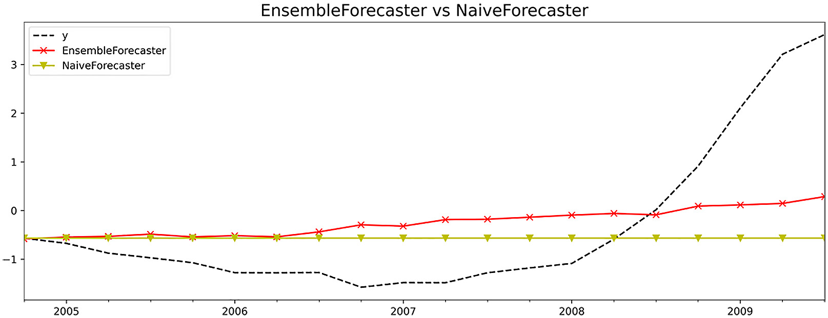
You can plot both forecasters for a visual comparison as well:
styles = ['k--','rx-','yv-']
for col, s in zip(y_hat, styles):
    y_hat[col].plot(style=s, label=col,
                    title='EnsembleForecaster vs NaiveForecaster' )
plt.legend();plt.show()
The preceding code should produce a plot showing all three time series for EnsembleForecaster, NaiveForecaster, and the test dataset.

Figure 12.16 – Plotting the two forecasters against the test data
Remember that neither of the models was optimized. Ideally, you can use k-fold cross-validation when training or a cross-validated grid search, as shown in the Optimizing a forecasting model with hyperparameter tuning recipe.
How it works...
The EnsembleForecaster class from sktime is similar to the VotingRegressor class in sklearn. Both are ensemble estimators that fit (train) several regressors and collectively, they produce a prediction through an aggregate function. Unlike VotingRegressor in sklearn, EnsembleForecaster allows you to change the aggfunc parameter to either mean (default), median, min, or max. When making a prediction with the predict method, only one prediction per one-step forecast horizon is produced. In other words, you will not get multiple predictions from each base regressor, but rather the aggregated value (for example, the mean) from all the base regressors.
Using a multivariate time series is made simple by using exogenous variables. Similarly, in statsmodels, an ARIMA or SARIMA model has an exog parameter. An ARIMA with exogenous variables is referred to as ARIMAX. Similarly, a seasonal ARIMA with exogenous variables is referred to as SARIMAX. To learn more about exogenous variables in statsmodels, you can refer to the documentation here: https://www.statsmodels.org/stable/endog_exog.html.
There's more...
The AutoEnsembleForecaster class in sktime behaves similar to the EnsembleForecaster class you used earlier. The difference is that the AutoEnsembleForecaster class will calculate the optimal weights for each of the regressors passed. The AutoEnsembleForecaster class has a regressor parameter that takes a list of regressors and estimates a weight for each class. In other words, not all regressors are treated equal. If none are provided, then the GradientBoostingRegressor class is used instead, with a default max_depth=5.
Using the same list of regressors, you will use AutoEnsembleForecaster and compare the results with NaiveForecaster and EnsembleForecaster:
from sktime.forecasting.compose import AutoEnsembleForecaster
auto = AutoEnsembleForecaster(forecasters=regressors,
                             method='feature-importance')
auto.fit(y=y_train, X=exog_train)
auto.weights_
>>
[0.1239225131192647,
 0.2634642533645639,
 0.2731867227890818,
 0.3394265107270897]
The order of the weights listed are based on the order from the regressor list provided. The highest weight was given to GradientBoostingRegressor at 34% followed by SupportVectorRegressor at 27%.
Using the predict method, let's compare the results:
y_hat['AutoEnsembleForecaster'] = auto.predict(fh=fh, X=exog_test)
evaluate(y_hat, y_train)
This should produce a DataFrame comparing all three forecasters:

Figure 12.17 – Evaluation of NaiveForecaster, EnsembleForecaster, and AutoEnsembleForecaster
Keep in mind that the number and type of regressors (or forecasters) used in both EnsembleForecaster and AutoEnsembleForecaster will have a significant impact on the overall quality. Keep in mind that none of these models have been optimized and are based on default hyperparameter values.
See also
To learn more about the AutoEnsembleForecaster class, you can read the official documentation here: https://www.sktime.org/en/stable/api_reference/auto_generated/sktime.forecasting.compose.AutoEnsembleForecaster.html.
To learn more about the EnsembleForecaster class, you can read the official documentation here: https://www.sktime.org/en/stable/api_reference/auto_generated/sktime.forecasting.compose.EnsembleForecaster.html.


