Search icon CANCEL
Subscription
0
Cart icon
Cart
Close icon
You have no products in your basket yet
Save more on your purchases!
Savings automatically calculated. No voucher code required
Arrow left icon
All Products
Best Sellers
New Releases
Books
Videos
Audiobooks
Learning Hub
Newsletters
Free Learning
Arrow right icon
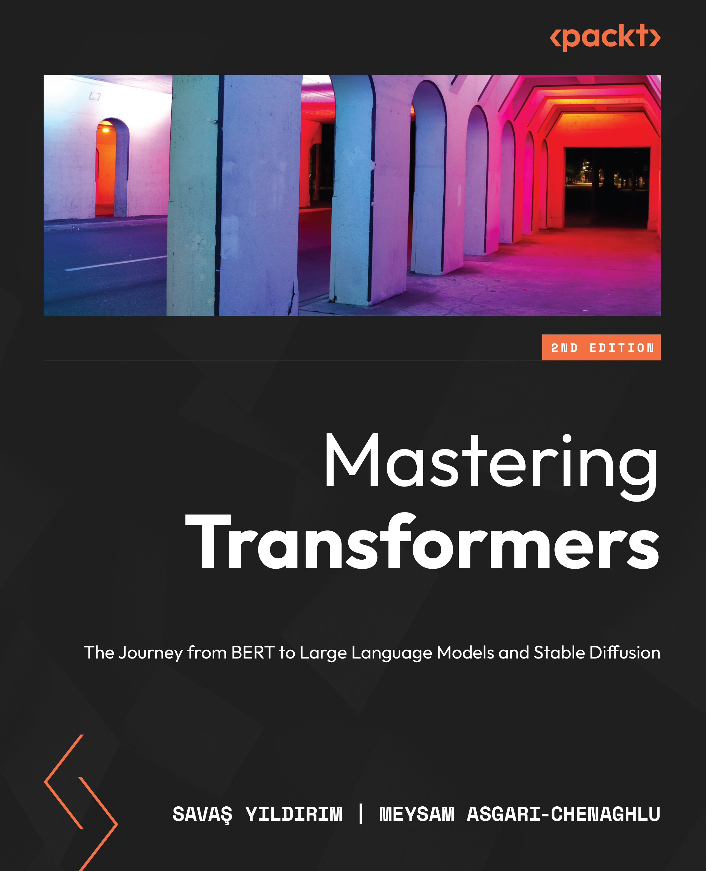
Mastering Transformers - Second Edition

Mastering Transformers: The Journey from BERT to Large Language Models and Stable Diffusion, Second Edition

By Savaş Yıldırım , Meysam Asgari- Chenaghlu
€32.99
Book Jun 2024 462 pages 2nd Edition
eBook
€32.99
Print
€41.99
Subscription
€14.99 Monthly
eBook
€32.99
Print
€41.99
Subscription
€14.99 Monthly

What do you get with eBook?

Product feature icon Instant access to your Digital eBook purchase
Product feature icon Download this book in EPUB and PDF formats
Product feature icon Access this title in our online reader with advanced features
Product feature icon DRM FREE - Read whenever, wherever and however you want
Buy Now
Table of content icon View table of contents Preview book icon Preview Book

Mastering Transformers - Second Edition

From Bag-of-Words to the Transformers

Over the past two decades, there have been significant advancements in the field of natural language processing (NLP). We have gone through various paradigms and have now arrived at the era of the Transformer architecture. These advancements have helped us represent words or sentences more effectively in order to solve NLP tasks. On the other hand, different use cases of merging textual inputs to other modalities, such as images, have emerged as well. Conversational artificial intelligence (AI) has seen the dawn of a new era. Chatbots were developed that act like humans by answering questions, describing concepts, and even solving mathematical equations step by step. All of these advancements happened in a very short period. One of the enablers of this huge advancement, without a doubt, was Transformer models.

Finding a cross-semantic understanding of different natural languages, natural languages and images, natural languages, and programming languages, and even in a broader sense, natural languages and almost any other modality, has opened a new gate for us to be able to use natural language as our primary input to perform many complex tasks in the field of AI. The easiest imaginable way is to just describe what we are looking for in a picture so the model will give us what we want (https://huggingface.co/spaces/CVPR/regionclip-demo):

Figure 1.1 – Zero-shot object detection with the prompt “A yellow apple”

Figure 1.1 – Zero-shot object detection with the prompt “A yellow apple”

The models have developed this skill through a process of ongoing learning and improvement. At first, distributional semantics and n-gram language models were traditionally utilized to understand the meanings of words and documents for years. It has been seen that these approaches had several limitations. On the other hand, with the rise of newer approaches for diffusing different modalities, modern approaches for training language models, especially large language models (LLMs), enabled many different use cases to come to life.

Classical deep learning (DL) architectures have significantly enhanced the performance of NLP tasks and have overcome the limitations of traditional approaches. Recurrent neural networks (RNNs), feed-forward neural networks (FFNNs), and convolutional neural networks (CNNs) are some of the widely used DL architectures for the solution. However, these models have also faced their own challenges. Recently, the Transformer model became standard, eliminating all the shortcomings of other models. It differed not only in solving a single monolingual task but also in the performance of multilingual, multitasking tasks. These contributions have made transfer learning (TL) more viable in NLP, which aims to make models reusable for different tasks or languages.

In this chapter, we will begin by examining the attention mechanism and provide a brief overview of the Transformer architecture. We will also highlight the distinctions between Transformer models and previous NLP models.

In this chapter, we will cover the following topics:

  • Evolution of NLP approaches
  • Recalling traditional NLP approaches
  • Leveraging DL
  • Overview of the Transformer architecture
  • Using TL with Transformers
  • Multimodal learning

Evolution of NLP approaches

Let us discuss how NLP has evolved over the past two decades as significant advancements have occurred in the field. Recently, the evolution has been primarily characterized by the transformative Transformer architecture. This architecture did not emerge out of thin air but, rather, evolved from various neural-based NLP approaches into an attention-based encoder-decoder architecture, which continues to evolve. In the past decade, the Transformer architecture and its variants have gained popularity due to the following developments:

  • Contextual word embeddings thanks to self-attention
  • Attention mechanisms, which overcome the problem of forcing input sentences to encode all information into one context vector
  • Better subword tokenization algorithms for handling unseen words or rare words
  • Injecting additional memory tokens into sentences, such as the paragraph ID in Doc2vec or a Classification ([CLS]) token in Bidirectional Encoder Representations from Transformers (BERT)
  • Parallelizable architectures that make for faster training and fine-tuning
  • Model compression (distillation, quantization, and so on)
  • TL capabilities: DL models can be easily adapted to new tasks or languages
  • Cross-lingual, multilingual, and multitasking learning capabilities
  • Multimodal training

For several years, traditional NLP approaches such as n-gram language models, TF-IDF-based models, BM25 information retrieval models, and one-hot encoded document-term matrices have been utilized to solve a range of NLP tasks, including sequence classification, language generation, and machine translation. However, these traditional approaches have limitations, such as difficulty in handling sparsity, rare words, and long-term dependencies. To address these challenges, we have developed DL-based approaches such as RNN, CNN, and FFNN, as well as several variants.

A document vector created by the TF-IDF model would have a size of more than 30,000 features. In 2013, word2vec, a two-layer FFNN word-encoder model, sorted out the dimensionality curse by generating compact and dense representations of words called word embeddings. This early model was able to create fast and efficient static word embeddings by converting unsupervised textual data into supervised data (self-supervised learning) through the prediction of target words using nearby neighboring words. Meanwhile, GloVe, another widely used and popular model, argued that count-based models can be better than neural models. It leverages both global and local statistics of a corpus to learn embeddings based on word-word co-occurrence statistics.

Word embeddings have proven effective for some syntactic and semantic tasks, as demonstrated in the following figure, which illustrates how the offsets between terms in the embeddings allow for vector-oriented reasoning. For example, we can discern the generalization of gender relations, a semantic relation, from the offset between the terms Man and Woman (Man -> Woman). Then, we can arithmetically estimate the vector of Actress by adding the vector of the term Actor and the offset calculated before. Likewise, we can learn the syntactic relationships, such as word plural forms. For instance, if the vectors of Actor, Actors, and Actress are given, we can estimate the vector of Actresses:

Figure 1.2 – Word embeddings offset for relationship extraction

Figure 1.2 – Word embeddings offset for relationship extraction

The representativeness of word embeddings has become a fundamental component for DL models such as RNNs or CNNs. The recurrent and convolutional architectures, respectively, started to be used as encoders and decoders in sequence-to-sequence (seq2seq) problems where each token is represented with an embedding. The main challenge with these early models was polysemous words (words with more than one meaning). The senses of the words are ignored since a single fixed representation is assigned to each word, which is an especially severe problem for sentence semantics.

Pioneering neural network models such as Universal Language Model Fine-tuning (ULMFiT) and Embeddings from Language Models (ELMo) were able to encode sentence-level information and alleviate polysemy issues, unlike static word embeddings. In this way, we have a new concept called contextual word embeddings.

The ULMFiT and ELMo approaches were based on LSTM (Long Short-Term Memory) networks, a variant of RNN. They also exploited the concept of pre-training and fine-tuning, which allows for TL by using pre-trained models trained on a general task with general textual datasets and fine-tuning them on a target task with supervision. This was a significant development because TL, which had previously been successful in image processing, was being applied for the first time in the field of NLP.

In the meantime, the idea of an attention mechanism (Neural Machine Translation by Jointly Learning to Align and Translate. Bahdanau et al., 2015) made a strong impression in the NLP field and achieved significant success, especially in seq2seq problems. Earlier methods would pass the last state (known as a context vector or thought vector) obtained from the entire input sequence to the output sequence without linking or elimination. Thanks to the attention mechanism, certain parts of the input can be associated with certain parts of the output.

In 2017, the Transformer-based encoder-decoder model was introduced and found to be successful due to its innovative use of the attention mechanism. The design is based on an FFNN by discarding RNN recurrency and using only attention mechanisms (Vaswani et al., Attention is All You Need, 2017). It overcame many difficulties that other approaches faced and has become a new paradigm. Throughout this book, you will be exploring and understanding how Transformer-based models work.

Recalling traditional NLP approaches

Although traditional models will soon become obsolete, they can always shed light on innovative designs. The most important of these is the distributional method, which is still used. Distributional semantics is a theory that explains the meaning of a word by analyzing its distributional evidence rather than relying on predefined dictionary definitions or other static resources. This approach suggests that words that frequently occur in similar contexts tend to have similar meanings. For example, words such as dog and cat often occur in similar contexts, suggesting that they may have related meanings. The idea was first proposed by Zellig S. Harris in his work, Distributional Structure of Words, in 1954. One of the benefits of using a distributional approach is that it allows researchers to track the semantic evolution of words over time or across different domains or senses of words, which is a task that is not possible using dictionary definitions alone.

For many years, traditional approaches to NLP have relied on Bag-of-Words (BoW) and n-gram language models to understand words and sentences. BoW approaches, also known as vector space models (VSMs), represent words and documents using one-hot encoding, a sparse representation method. These one-hot encoding techniques have been used to solve a variety of NLP tasks, such as text classification, word similarity, semantic relation extraction, and word-sense disambiguation. On the other hand, n-gram language models assign probabilities to sequences of words, which can be used to calculate the likelihood that a given sequence belongs to a corpus or to generate random sequences based on a given corpus.

Along with these models, in order to assign importance to a term, the Term Frequency (TF) and the Inverse Document Frequency (IDF) metrics are often used. IDF helps to reduce the weight of high-frequency words, such as stop words and functional words, which have little discriminatory power in understanding the content of a document. The discriminatory power of a term also depends on the domain – for example, a list of articles about DL is likely to have the word network in almost every document. It would not be a surprise to see the term network in the domain data. The Document Frequency (DF) of a word is calculated by counting the number of documents in which it appears, and this can be used to scale down the weights of all terms. The TF is simply the raw count of a term in a document.

Some of the advantages and disadvantages of a TF-IDF-based BoW model are listed as follows:

Advantages

Disadvantages

  • Easy to implement
  • Human-interpretable results
  • Domain adaptation
  • Dimensionality curse
  • No solution for unseen words
  • Hardly captures semantic relations (is-a, has-a, synonym)
  • Ignores word order
  • Slow for large vocabulary

Table 1.1 – Advantages and disadvantages of a TF-IDF BoW model

Using a BoW approach to represent a small sentence can be impractical because it involves representing each word in the dictionary as a separate dimension in a vector, regardless of whether it appears in the sentence or not. This can result in a high-dimensional vector with many zero cells, making it difficult to work with and requiring a large amount of memory to store.

Latent semantic analysis (LSA) has been widely used to overcome the dimensionality problem of the BoW model. It is a linear method that captures pairwise correlations between terms. LSA-based probabilistic methods can still be considered as a single layer of hidden topic variables. However, current DL models include multiple hidden layers, with billions of parameters. In addition to that, Transformer-based models showed that they can discover latent representations much better than such traditional models.

The traditional pipeline for NLP tasks begins with a series of preparation steps, such as tokenization, stemming, noun phrase detection, chunking, and stop-word elimination. After these steps are completed, a document-term matrix is constructed using a weighting schema, with TF-IDF being the most popular choice. This matrix can then be used as input for various machine learning (ML) pipelines, including sentiment analysis, document similarity, document clustering, and measuring the relevancy score between a query and a document. Similarly, terms can be represented as a matrix and used as input for token classification tasks, such as named entity recognition and semantic relation extraction. The classification phase typically involves the application of supervised ML algorithms, such as support vector machines (SVMs), random forests, logistic regression, naive Bayes, and multiple learners (boosting or bagging).

Language modeling and generation

Traditional approaches to language generation tasks often rely on n-gram language models, also known as Markov processes. These are stochastic models that estimate the probability of a word (event) based on a subset of previous words. There are three main types of n-gram models: unigram, bigram, and n-gram (generalized). Let us look at these in more detail:

  • Unigram models assume that all words are independent and do not form a chain. The probability of a word in a vocabulary is simply calculated by its frequency in the total word count.
  • Bigram models, also known as first-order Markov processes, estimate the probability of a word based on the previous word. This probability is calculated by the ratio of the joint probability of two consecutive words to the probability of the first word.
  • N-gram models, also known as N-order Markov processes, estimate the probability of a word based on the previous n-1 words.

We have already discussed the paradigms underlying traditional NLP models in the Recalling traditional NLP approaches subsection and provided a brief introduction. We will now move on to discuss how neural language models have impacted the field of NLP and how they have addressed the limitations of traditional models.

Leveraging DL

For decades, we have witnessed successful architectures, especially in word and sentence representation. Neural network-based language models have been effective in addressing feature representation and language modeling problems because they allow for the training of more advanced neural architectures on large datasets, which enables the learning of compact, high-quality representations of language.

In 2013, the word2vec model introduced a simple and effective architecture for learning continuous word representations that outperformed other models on a variety of syntactic and semantic language tasks, such as sentiment analysis, paraphrase detection, and relation extraction. The low computational complexity of word2vec has also contributed to its popularity. Due to the success of embedding methods, word embedding representation has gained attraction and is now widely used in modern NLP models.

Word2vec and similar models learn word embeddings through the use of a prediction-based neural architecture based on nearby word predictions. This approach differs from traditional BoW methods that rely on count-based techniques for capturing distributional semantics. The authors of the GloVe model have addressed the question of whether count-based or prediction-based methods are better for distributional word representations and claimed that the two approaches are not significantly different. FastText is another widely used model that incorporates subword information by representing each word as a bag of character n-grams, with each n-gram represented by a constant vector. Words are then represented as the sum of their sub-vectors, an idea first introduced by H. Schütze in 1993. This allows FastText to compute word representations even for unseen words (or rare words) and learn the internal structure of words, such as suffixes and affixes, which is particularly useful for morphologically rich languages. Likewise, modern Transformer architectures exploit incorporating subword information and use various subword tokenization methods, such as WordPiece, SentencePiece, or Byte-Pair Encoding (BPE).

Let us quickly discuss popular RNN models.

Considering the word order with RNN models

Traditional BoW models do not consider word order because they treat all words as individual units and place them in a basket. RNN models, on the other hand, learn the representation of each token (word) by cumulatively incorporating the information of previous tokens, and the final token ultimately provides the representation of the entire sentence.

Like other neural network models, RNN models process tokens produced by a tokenization algorithm that breaks down raw text into atomic units, known as tokens. These tokens are then associated with numeric vectors, called token embeddings, which are learned during training. Alternatively, we can use well-known word-embedding algorithms, such as word2vec or FastText, to generate these token embeddings in advance.

Here is a simple illustration of an RNN architecture for the sentence The cat is sad., where x0 is the vector embeddings of the, x1 is the vector embeddings of cat, and so forth. Figure 1.3 illustrates an RNN being unfolded into a full deep neural network (DNN). Unfolding means that we associate a layer to each word. For the The cat is sad. sequence, we take care of a sequence of five tokens. The hidden state in each layer acts as the memory of the network and is shared between the steps. It encodes information about what happened in all previous timesteps and in the current timestep. This is represented in the following diagram:

Figure 1.3 – An RNN architecture

Figure 1.3 – An RNN architecture

The following are some advantages of an RNN architecture:

  • Variable-length input: The capacity to work on variable-length input, no matter the size of the sentence being input. We can feed the network with sentences of 3 or 300 words without changing the parameter.
  • Caring about word order: It processes the sequence word by word in order, caring about the word position.
  • Suitable for working in various modes: We can train a machine translation model or sentiment analysis using the same recurrency paradigm. Both architectures would be based on an RNN:
    • One-to-many mode: RNN can be redesigned in a one-to-many model for language generation or music generation. (e.g., a word -> its definition in a sentence)
    • Many-to-one mode: It can be used for text classification or sentiment analysis (e.g., a sentence as a list of words -> sentiment score)
    • Many-to-many mode: The use of many-to-many models is to solve encoder-decoder problems such as machine translation, question answering, and text summarization or Named Entity Recognition (NER)-like sequence labeling problems

The disadvantages of an RNN architecture are listed here:

  • Long-term dependency problem: When we process a very long document and try to link the terms that are far from each other, we need to care about and encode all irrelevant other terms between these terms.
  • Prone to exploding or vanishing gradient problems: When working on long documents, updating the weights of the very first words is a big deal, which makes a model untrainable due to a vanishing gradient problem.
  • Hard to apply parallelizable training: Parallelization breaks the main problem down into a smaller problem and executes the solutions at the same time, but RNN follows a classic sequential approach. Each layer strongly depends on previous layers, which makes parallelization impossible.
  • The computation is slow as the sequence is long: An RNN could be very efficient for short text problems. It processes longer documents very slowly, besides the long-term dependency problem.

Although an RNN can theoretically attend to the information many timesteps before, in the real world, problems such as long documents and long-term dependencies are impossible to discover. Long sequences are represented within many deep layers. These problems have been addressed by many studies, some of which are outlined here:

  • Hochreiter and Schmidhuber. Long Short-term Memory. 1997.
  • Bengio et al. Learning long-term dependencies with gradient descent is difficult. 1993.
  • K. Cho et al. Learning phrase representations using RNN encoder-decoder for statistical machine translation. 2014.

LSTMs and gated recurrent units

LSTM networks (Schmidhuber, 1997) and gated recurrent units (GRUs) (Cho, 2014) are types of RNNs that are designed to address the problem of long-term dependencies. One key feature of LSTMs is the use of a cell state, which is a horizontal sequence line located above the LSTM unit and controlled by specialized gates that handle forget, insert, or update operations. The complex structure of an LSTM is shown in the following diagram:

Figure 1.4 – An LSTM unit

Figure 1.4 – An LSTM unit

The design is able to decide the following:

  • What kind of information we will store in the cell state
  • Which information will be forgotten or deleted

In the original RNN, in order to learn the state of any token, it recurrently processes the entire state of previous tokens. Carrying entire information from earlier timesteps leads to vanishing gradient problems, which makes the model untrainable. You can think of it this way: the difficulty of carrying information increases exponentially with each step. For example, let’s say that carrying information with the previous token is 2 units of difficulty; with the 2 previous tokens, it would be 4 units, and with 10 previous tokens, it becomes 1,024 units of difficulty.

The gate mechanism in LSTM allows the architecture to skip some unrelated tokens at a certain timestep or remember long-range states to learn the current token state. The GRU is similar to an LSTM in many ways, the main difference being that a GRU does not use the cell state. Rather, the architecture is simplified by transferring the functionality of the cell state to the hidden state, and it only includes two gates: an update gate and a reset gate. The update gate determines how much information from the previous and current timesteps will be pushed forward. This feature helps the model keep relevant information from the past, which minimizes the risk of a vanishing gradient problem as well. The reset gate detects the irrelevant data and makes the model forget it.

In a seq2seq pipeline with traditional RNNs, it was necessary to compress all the information into a single representation in the input data. However, this can make it difficult for the output tokens to focus on specific parts of the input tokens. Bahdanau’s attention mechanism was first applied to RNNs and has shown to be effective in addressing this issue and has become a key concept in the Transformer architecture. We will examine how the Transformer architecture uses attention in more detail later in the book.

Contextual word embeddings and TL

Traditional word embeddings such as word2vec were important components of many neural language understanding models. However, using these embeddings in a language modeling task would result in the same representation for the word bank regardless of the context in which it appears. For example, the word bank would have the same embedding whether it refers to a financial institution or side of a river with traditional vectors. At this point, context is important for humans as well as machines to understand the meaning of a word.

In this line, ELMo and ULMFiT were the pioneering models that achieved contextual word embeddings and efficient TL in NLP. They got good results on a variety of language understanding tasks, such as question answering, NER, relation extraction, and so forth. These contextual embeddings capture both the meaning of a word and the context in which it appears. Unlike traditional word embeddings, which use a static representation for each word, they use bi-directional LSTM to encode a word by considering the entire sentence in which it appears.

They demonstrated that pre-trained word embeddings can be reused for other NLP tasks once the pre-training has been completed. ULMFiT, in particular, was successful in applying TL to NLP tasks. At that time, TL was already commonly used in computer vision, but existing NLP approaches still required task-specific modifications and training from scratch. ULMFiT introduced an effective TL method that can be applied to any NLP task and also demonstrated techniques for fine-tuning a language model. The ULMFiT process consists of three stages. The first stage is the pre-training of a general domain language model on a large corpus to capture general language features at different layers. The second stage involves fine-tuning the pre-trained language model on a target task dataset using discriminative fine-tuning to learn task-specific features. The final stage involves fine-tuning the classifier on the target task with gradual unfreezing. This approach maintains low-level representations while adapting to high-level ones.

Now, we finally come to our main topic—Transformers!

Overview of the Transformer architecture

Transformer models have received immense interest because of their effectiveness in an enormous range of NLP problems, from text classification to text generation. The attention mechanism is an important part of these models and plays a very crucial role. Before Transformer models, the attention mechanism was proposed as a helper for improving conventional DL models such as RNNs. To understand Transformers and their impact on NLP, we will first study the attention mechanism.

Attention mechanism

The attention mechanism allowed for the creation of a more advanced model by connecting specific tokens in the input sequence to specific tokens in the output sequence. For instance, suppose you have the keyword phrase Canadian Government in the input sentence for an English-to-Turkish translation task. In the output sentence, the Kanada Hükümeti tokens make strong connections with the input phrase and establish a weaker connection with the remaining words in the input, as illustrated in the following figure:

Figure 1.5 – Sketchy visualization of an attention mechanism

Figure 1.5 – Sketchy visualization of an attention mechanism

This mechanism makes models more successful in seq2seq tasks such as translation, question answering, and text summarization.

One of the first variations of the attention mechanism was proposed by Bahdanau et al. (2015). This mechanism is based on the fact that RNN-based models such as GRUs or LSTMs have an information bottleneck on tasks such as neural machine translation (NMT). These encoder-decoder-based models get the input in the form of a token ID and process it in a recurrent fashion (encoder). Afterward, the processed intermediate representation is fed into another recurrent unit (decoder) to extract the results. This avalanche-like information is like a rolling ball that consumes all the information, and rolling it out is hard for the decoder part because it does not see all the dependencies and only gets the intermediate representation (context vector) as input.

To align this mechanism, Bahdanau proposed an attention mechanism to use weights on intermediate hidden values. These weights align the amount of attention that a model must pay to the input in each decoding step. Such wonderful guidance assists models in specific tasks such as NMT, which is a many-to-many task. Different attention mechanisms have been proposed with different improvements. Additive, multiplicative, general, and dot-product attention appear within the family of these mechanisms. The latter, which is a modified version with a scaling parameter, is noted as scaled dot-product attention. This specific attention type is the foundation of Transformers models and is called a multi-head attention mechanism. Additive attention is also what was introduced earlier as a notable change in NMT tasks. You can see an overview of the different types of attention mechanisms here:

Name

Attention score function

Content-based attention

Additive

Location-based

General

Dot-product

Scaled dot-product

Table 1.2 – Types of attention mechanisms

In Table 1.2, h and s represent the hidden state and state itself, respectively, while W denotes the weights specific to the attention mechanism.

Since attention mechanisms are not specific to NLP; they are also used in different use cases in various fields, from computer vision to speech recognition. The following figure shows a visualization of a multimodal approach trained for neural image captioning (K Xu et al., Show, Attend and Tell: Neural Image Caption Generation with Visual Attention, 2015):

Figure 1.6 – Attention in Computer Vision

Figure 1.6 – Attention in Computer Vision

Another example is as follows:

Figure 1.7 – Another example for Attention mechanism in computer vision

Figure 1.7 – Another example for Attention mechanism in computer vision

Next, let’s understand multi-head attention mechanisms.

Multi-head attention mechanisms

The multi-head attention mechanism that is shown in the following diagram is an essential part of the Transformer architecture:

Figure 1.8 – Multi-head attention mechanism

Figure 1.8 – Multi-head attention mechanism

Before jumping into scaled dot-product attention mechanisms, it’s better to get a good understanding of self-attention. Self-attention, as shown in Figure 1.8, is a basic form of a scaled self-attention mechanism. This mechanism uses an input matrix and produces an attention score between various items

Q in Figure 1.9 is known as the query, K is known as the key, and V is noted as the value. Three types of matrices shown as theta, phi, and g are multiplied by X before producing Q, K, and V. The multiplied result between the query (Q) and key (K) yields an attention score matrix. This can also be seen as a database where we use the query and keys in order to find out how various items are related in terms of numeric evaluation. Multiplication of the attention score and the V matrix produces the final result of this type of attention mechanism. The main reason for it being called self-attention is because of its unified input X (Q, K, and V are computed from X). You can see all this depicted in the following diagram:

Figure 1.9 – Mathematical representation for the attention mechanism (diagram inspiration from https://blogs.oracle.com/datascience/multi-head-self-attention-in-nlp)

Figure 1.9 – Mathematical representation for the attention mechanism (diagram inspiration from https://blogs.oracle.com/datascience/multi-head-self-attention-in-nlp)

A scaled dot-product attention mechanism is very similar to a self-attention (dot-product) mechanism except it uses a scaling factor. The multi-head part, on the other hand, ensures the model can look at various aspects of input at all levels. Transformer models attend to encoder annotations and the hidden values from past layers. The architecture of the Transformer model does not have a recurrent step-by-step flow; instead, it uses positional encoding to receive information about the position of each token in the input sequence. The concatenated values of the embeddings (randomly initialized) and the fixed values of positional encoding are the input fed into the layers in the first encoder part and are propagated through the architecture, as illustrated in the following diagram:

Figure 1.10 – A Transformer architecture

Figure 1.10 – A Transformer architecture

The positional information is obtained by evaluating sine and cosine waves at different frequencies. An example of positional encoding is visualized in the following figure:

Figure 1.11 – Positional encoding

Figure 1.11 – Positional encoding

A good example of performance for the Transformer architecture and the scaled dot-product attention mechanism is given in the following figure:

Figure 1.12 – Attention mapping for Transformers

Figure 1.12 – Attention mapping for Transformers

The word it refers to different entities in different contexts. As seen in Figure 1.12, it refers to cat. If we changed angry to stale, it would refer to food. Another improvement made by using a Transformer architecture is in parallelism. Conventional sequential recurrent models such as LSTMs and GRUs do not have such capabilities because they process the input token by token. Feed-forward layers, on the other hand, speed up a bit more because single matrix multiplication is far faster than a recurrent unit. Stacks of multi-head attention layers gain a better understanding of complex sentences.

On the decoder side of the attention mechanism, a very similar approach to the encoder is utilized with small modifications. A multi-head attention mechanism is the same, but the output of the encoder stack is also used. This encoding is given to each decoder stack in the second multi-head attention layer. This little modification introduces the output of the encoder stack while decoding. This modification lets the model be aware of the encoder output while decoding and, at the same time, helps it during training to have a better gradient flow over various layers. The final softmax layer at the end of the decoder layer is used to provide outputs for various use cases such as NMT, for which the original Transformer architecture was introduced.

This architecture has two inputs, noted as inputs and outputs (shifted right). One is always present (inputs) in both training and inference, while the other is just present in training and inference, which is produced by the model. The reason we do not use model predictions in inference is to stop the model from going too wrong by itself. But what does it mean? Imagine a neural translation model trying to translate a sentence from English to French—at each step, it makes a prediction for a word, and it uses that predicted word to predict the next one. But if it goes wrong at some step, all the subsequent predictions will be wrong, too. To stop the model from going wrong like this, we provide the correct words as a shifted-right version.

A visual example of a Transformer model is given in the following diagram. It shows a Transformer model with two encoders and two decoder layers. The Add & Normalize layer from this diagram adds and normalizes the input it takes from the Feed Forward layer:

Figure 1.13 – Transformer model (inspiration from http://jalammar.github.io/illustrated-Transformer/)

Figure 1.13 – Transformer model (inspiration from http://jalammar.github.io/illustrated-Transformer/)

Another major improvement that is used by a Transformer-based architecture is based on a simple universal text compression scheme to prevent unseen tokens on the input side. This approach, which takes place by using different methods such as byte-pair encoding and sentence-piece encoding, improves a Transformer’s performance in dealing with unseen tokens. It also guides the model when the model encounters morphologically close tokens. Such tokens were unseen in the past and are rarely used in the training, and yet, an inference might be seen. In some cases, chunks of it are seen in training; the latter happens in the case of morphologically rich languages such as Turkish, German, Czech, and Latvian. For example, a model might see the word training but not trainings. In such cases, it can tokenize trainings as training+s. These two are commonly seen when we look at them as two parts.

Transformer-based models have quite common characteristics—for example, they are all based on this original architecture with differences in the steps they use and don’t use. In some cases, minor differences are made—for example, improvements to the multi-head attention mechanism taking place.

Now, we will discuss how to apply TL within Transformers in the following section.

Using TL with Transformers

TL is a field of AI that aims to make models reusable for different tasks—for example, a model trained on a given task such as A is reusable (fine-tuning) on a different task such as B. In an NLP field, this is achievable by using Transformer-like architectures that can capture the understanding of language itself by language modeling. Such models are called language models—they provide a model for the language they have been trained on. TL is not a new technique, and it has been used in various fields such as computer vision. ResNet, Inception, Visual Geometry Group (VGG), and EfficientNet are examples of such models that can be used as pre-trained models able to be fine-tuned on different computer vision tasks.

Shallow TL using models such as Word2vec, GloVe, and Doc2vec is also possible in NLP. It is called shallow because there is no model to be transferred behind this kind of TL and instead, the pre-trained vectors for words/tokens are transferred. You can use these token- or document-embedding models followed by a classifier or use them combined with other models such as RNNs instead of using random embeddings.

TL in NLP using Transformer models is also possible because these models can learn a language itself without any labeled data. Language modeling is a task used to train transferable weights for various problems. Masked language modeling is one of the methods used to learn a language itself. As with Word2vec’s window-based model for predicting center tokens, in masked language modeling, a similar approach takes place but with key differences. Given a probability, each word is masked and replaced with a special token such as [MASK]. The language model (a Transformer-based model, in our case) must predict the masked words. Instead of using a window, unlike with Word2vec, a whole sentence is given, and the output of the model must be the same sentence with masked words filled.

One of the first models that used the Transformer architecture for language modeling is BERT, which is based on the encoder part of the Transformer architecture. Masked language modeling is accomplished by BERT using the same method described before and after training a language model. BERT is a transferable language model for different NLP tasks such as token classification, sequence classification, or even question answering.

Each of these tasks is a fine-tuning task for BERT once a language model is trained. BERT is best known for its key characteristics on the base Transformer encoder model, and by altering these characteristics, different versions of it—small, tiny, base, large, and extra-large—are proposed. Contextual embedding enables a model to have the correct meaning of each word based on the context in which it is given—for example, the word cold can have different meanings in two different sentences: cold-hearted killer and cold weather. The number of layers at the encoder part, the input dimension, the output embedding dimension, and the number of multi-head attention mechanisms are key characteristics, as illustrated in the following figure:

Figure 1.14 – Pre-training and fine-tuning procedures for BERT (image inspiration from J. Devlin et al., Bert: Pre-training of deep bidirectional Transformers for language understanding, 2018)

Figure 1.14 – Pre-training and fine-tuning procedures for BERT (image inspiration from J. Devlin et al., Bert: Pre-training of deep bidirectional Transformers for language understanding, 2018)

As you can see in Figure 1.14, the pre-training phase also consists of another objective known as next-sentence prediction. As we know, each document is composed of sentences followed by each other, and another important part of training a model to grasp the language is to understand the relationships of sentences to each other—in other words, whether they are related or not. To achieve these tasks, BERT introduced special tokens such as [CLS] and [SEP]. A [CLS] token is an initially meaningless token used as the starting token for all tasks, and it contains all information about the sentence. In sequence-classification tasks such as next sentence prediction (NSP), a classifier on top of the output of this token (output position of 0) is used. It is also useful in evaluating the sense of a sentence or capturing its semantics—for example, when using a Siamese BERT model, comparing these two [CLS] tokens for different sentences by a metric such as cosine similarity is very helpful. On the other hand, [SEP] is used to distinguish between two sentences, and it is only used to separate two sentences. After pre-training, if someone aims to fine-tune BERT on a sequence classification task such as sentiment analysis, they will use a classifier on top of the output embedding of [CLS]. It is also notable that all TL models can be frozen during fine-tuning or freed; frozen means seeing all weights and biases inside the model as constants and stopping training on them. In the example of sentiment analysis, just the classifier will be trained, not the model if it is frozen.

In the next section, you will learn about multimodal learning. You will also get familiar with different architectures that use this learning paradigm with respect to Transformers.

Multimodal learning

Multimodal learning is a general topic in AI that refers to solutions where the associated data is not in a single modality (only image, only text, etc.) but instead, more than one modality is involved. As an example, consider a problem where both an image and text are involved as input or output. Another example can be a cross-modality problem where the input and output modalities are not the same.

Before jumping into multimodal learning using Transformers, it is useful to describe how they can be used for images as well. Transformers get the input in the form of a sequence but, unlike text, images are not 1D sequences. One of the approaches in this field tries to convert the image into patches. Each patch is linearly projected into a vector shape and positional encoding is applied.

Figure 1.15 shows the architecture of the Vision Transformer (ViT) and how it works:

Figure 1.15 – Vision Transformer (https://ai.googleblog.com/2020/12/transformers-for-image-recognition-at.html)

Figure 1.15 – Vision Transformer (https://ai.googleblog.com/2020/12/transformers-for-image-recognition-at.html)

Like architectures such as BERT, a classification head can be applied for tasks such as image classification. However, other use cases and applications can be drawn from this approach as well.

Using a Transformer for images or text separately can create a nice model that can understand text or images. But if we want to have a model that can understand both at the same time and create a link between text and images, it would require training both with constraints. Contrastive Language–Image Pre-training (CLIP) is one of the models that can understand images and text. It can be used for semantic search where the input can be a text/image and the output is a text/image.

The next figure shows how the CLIP model is trained by using a dual encoder:

Figure 1.16 – CLIP model contrastive pre-training (https://openai.com/blog/clip/)

Figure 1.16 – CLIP model contrastive pre-training (https://openai.com/blog/clip/)

As it is clear from the CLIP architecture, it will be very useful for zero-shot prediction for text and image modalities. DALL-E and diffusion-based models such as Stable Diffusion are in this category.

The Stable Diffusion pipeline is shown in the next figure:

Figure 1.17 – Stable Diffusion pipeline

Figure 1.17 – Stable Diffusion pipeline

The preceding diagram can also be viewed at https://www.tensorflow.org/tutorials/generative/generate_images_with_stable_diffusion, and the license is as follows: https://creativecommons.org/licenses/by/4.0/.

For example, Stable Diffusion uses a text encoder to convert text into dense vectors, and, accordingly, a diffusion model tries to create a vector representation of the respective image. The decoder tries to decode this vector representation, and finally, an image with semantic similarity to the text input is produced.

Multimodal learning not only helps us use different modalities for tasks that are always related to image-text but it can also be used in many different modalities combined with text, such as speech, numerical data, and graphs.

Summary

With this, we have reached the end of the chapter. You should now understand the evolution of NLP methods and approaches, from BoW to Transformers. We looked at how to implement BoW, RNN, and CNN-based approaches and understood what Word2vec is and how it helps improve the conventional DL-based methods using shallow TL. We also investigated the foundation of the Transformer architecture, with BERT as an example. We learned about TL and how it is utilized by BERT. We also described the general idea behind multimodal learning and provided a quick introduction to ViT. Models such as CLIP and Stable Diffusion were also described.

At this point, we have learned the basic information that is necessary to continue to the next chapters. We understand the main idea behind Transformer-based architectures and how TL can be applied using this architecture.

In the next chapter, we will see how it is possible to run a simple Transformer example from scratch. The related information about the installation steps will be given, and working with datasets and benchmarks will also be investigated in detail.

References

  • Mikolov, T., Chen, K., Corrado, G., and Dean, J. (2013). Efficient estimation of word representations in vector space. arXiv preprint arXiv:1301.3781.
  • Bahdanau, D., Cho, K., and Bengio, Y. (2014). Neural machine translation by jointly learning to align and translate. arXiv preprint arXiv:1409.0473.
  • Pennington, J., Socher, R., and Manning, C. D. (2014, October). GloVe: Global vectors for word representation. In Proceedings of the 2014 conference on empirical methods in natural language processing (EMNLP) (pp. 1532-1543).
  • Hochreiter, S. and Schmidhuber, J. (1997). Long short-term memory. Neural computation, 9(8), 1735-1780.
  • Bengio, Y., Simard, P, and Frasconi, P. (1994). Learning long-term dependencies with gradient descent is difficult. IEEE transactions on neural networks, 5(2), 157-166.
  • Cho, K., et al. (2014). Learning phrase representations using RNN encoder-decoder for statistical machine translation. arXiv preprint arXiv:1406.1078.
  • Kim, Y. (2014). Convolutional neural networks for sentence classification. CoRR abs/1408.5882 (2014). arXiv preprint arXiv:1408.5882.
  • Vaswani, A., et al. (2017). Attention is all you need. arXiv preprint arXiv:1706.03762.
  • Devlin, J., Chang, M. W., Lee, K., and Toutanova, K. (2018). Bert: Pre-training of deep bidirectional Transformers for language understanding. arXiv preprint arXiv:1810.04805.
  • Alammar (2022). The Illustrated stable diffusion. https://jalammar.github.io/illustrated-stable-diffusion/
  • Zhong, Y., et al. (2022). Regionclip: Region-based language-image pretraining. In Proceedings of the IEEE/CVF Conference on Computer Vision and Pattern Recognition (pp. 16793-16803).
  • Dosovitskiy, A., et al. (2020). An image is worth 16x16 words: Transformers for image recognition at scale. arXiv preprint arXiv:2010.11929.
  • Radford, A., et al. (2021, July). Learning transferable visual models from natural language supervision. In International Conference on Machine Learning (pp. 8748-8763). PMLR.
Left arrow icon Right arrow icon
Download code icon Download Code

Key benefits

  • Understand the complexity of deep learning architecture and transformers architecture
  • Create solutions to industrial natural language processing (NLP) and computer vision (CV) problems
  • Explore challenges in the preparation process, such as problem and language-specific dataset transformation
  • Purchase of the print or Kindle book includes a free PDF eBook

Description

Transformer-based language models such as BERT, T5, GPT, DALL-E, and ChatGPT have dominated NLP studies and become a new paradigm. Thanks to their accurate and fast fine-tuning capabilities, transformer-based language models have been able to outperform traditional machine learning-based approaches for many challenging natural language understanding (NLU) problems. Aside from NLP, a fast-growing area in multimodal learning and generative AI has recently been established, showing promising results. Mastering Transformers will help you understand and implement multimodal solutions, including text-to-image. Computer vision solutions that are based on transformers are also explained in the book. You’ll get started by understanding various transformer models before learning how to train different autoregressive language models such as GPT and XLNet. The book will also get you up to speed with boosting model performance, as well as tracking model training using the TensorBoard toolkit. In the later chapters, you’ll focus on using vision transformers to solve computer vision problems. Finally, you’ll discover how to harness the power of transformers to model time series data and for predicting. By the end of this transformers book, you’ll have an understanding of transformer models and how to use them to solve challenges in NLP and CV.

What you will learn

Focus on solving simple-to-complex NLP problems with Python Discover how to solve classification/regression problems with traditional NLP approaches Train a language model and explore how to fine-tune models to the downstream tasks Understand how to use transformers for generative AI and computer vision tasks Build transformer-based NLP apps with the Python transformers library Focus on language generation such as machine translation and conversational AI in any language Speed up transformer model inference to reduce latency

Product Details

Country selected

Publication date : Jun 3, 2024
Length 462 pages
Edition : 2nd Edition
Language : English
ISBN-13 : 9781837633784
Category :
Languages :
Concepts :

What do you get with eBook?

Product feature icon Instant access to your Digital eBook purchase
Product feature icon Download this book in EPUB and PDF formats
Product feature icon Access this title in our online reader with advanced features
Product feature icon DRM FREE - Read whenever, wherever and however you want
Buy Now

Product Details


Publication date : Jun 3, 2024
Length 462 pages
Edition : 2nd Edition
Language : English
ISBN-13 : 9781837633784
Category :
Languages :
Concepts :

Table of Contents

25 Chapters
Preface Chevron down icon Chevron up icon
1. Part 1: Recent Developments in the Field, Installations, and Hello World Applications Chevron down icon Chevron up icon
2. Chapter 1: From Bag-of-Words to the Transformers Chevron down icon Chevron up icon
3. Chapter 2: A Hands-On Introduction to the Subject Chevron down icon Chevron up icon
4. Part 2: Transformer Models: From Autoencoders to Autoregressive Models Chevron down icon Chevron up icon
5. Chapter 3: Autoencoding Language Models Chevron down icon Chevron up icon
6. Chapter 4: From Generative Models to Large Language Models Chevron down icon Chevron up icon
7. Chapter 5: Fine-Tuning Language Models for Text Classification Chevron down icon Chevron up icon
8. Chapter 6: Fine-Tuning Language Models for Token Classification Chevron down icon Chevron up icon
9. Chapter 7: Text Representation Chevron down icon Chevron up icon
10. Chapter 8: Boosting Model Performance Chevron down icon Chevron up icon
11. Chapter 9: Parameter Efficient Fine-Tuning Chevron down icon Chevron up icon
12. Part 3: Advanced Topics Chevron down icon Chevron up icon
13. Chapter 10: Large Language Models Chevron down icon Chevron up icon
14. Chapter 11: Explainable AI (XAI) in NLP Chevron down icon Chevron up icon
15. Chapter 12: Working with Efficient Transformers Chevron down icon Chevron up icon
16. Chapter 13: Cross-Lingual and Multilingual Language Modeling Chevron down icon Chevron up icon
17. Chapter 14: Serving Transformer Models Chevron down icon Chevron up icon
18. Chapter 15: Model Tracking and Monitoring Chevron down icon Chevron up icon
19. Part 4: Transformers beyond NLP Chevron down icon Chevron up icon
20. Chapter 16: Vision Transformers Chevron down icon Chevron up icon
21. Chapter 17: Multimodal Generative Transformers Chevron down icon Chevron up icon
22. Chapter 18: Revisiting Transformers Architecture for Time Series Chevron down icon Chevron up icon
23. Index Chevron down icon Chevron up icon
24. Other Books You May Enjoy Chevron down icon Chevron up icon

Customer reviews

Top Reviews
Rating distribution
Empty star icon Empty star icon Empty star icon Empty star icon Empty star icon 0
(0 Ratings)
5 star 0%
4 star 0%
3 star 0%
2 star 0%
1 star 0%
Top Reviews
No reviews found
Get free access to Packt library with over 7500+ books and video courses for 7 days!
Start Free Trial

FAQs

How do I buy and download an eBook? Chevron down icon Chevron up icon

Where there is an eBook version of a title available, you can buy it from the book details for that title. Add either the standalone eBook or the eBook and print book bundle to your shopping cart. Your eBook will show in your cart as a product on its own. After completing checkout and payment in the normal way, you will receive your receipt on the screen containing a link to a personalised PDF download file. This link will remain active for 30 days. You can download backup copies of the file by logging in to your account at any time.

If you already have Adobe reader installed, then clicking on the link will download and open the PDF file directly. If you don't, then save the PDF file on your machine and download the Reader to view it.

Please Note: Packt eBooks are non-returnable and non-refundable.

Packt eBook and Licensing When you buy an eBook from Packt Publishing, completing your purchase means you accept the terms of our licence agreement. Please read the full text of the agreement. In it we have tried to balance the need for the ebook to be usable for you the reader with our needs to protect the rights of us as Publishers and of our authors. In summary, the agreement says:

  • You may make copies of your eBook for your own use onto any machine
  • You may not pass copies of the eBook on to anyone else
How can I make a purchase on your website? Chevron down icon Chevron up icon

If you want to purchase a video course, eBook or Bundle (Print+eBook) please follow below steps:

  1. Register on our website using your email address and the password.
  2. Search for the title by name or ISBN using the search option.
  3. Select the title you want to purchase.
  4. Choose the format you wish to purchase the title in; if you order the Print Book, you get a free eBook copy of the same title. 
  5. Proceed with the checkout process (payment to be made using Credit Card, Debit Cart, or PayPal)
Where can I access support around an eBook? Chevron down icon Chevron up icon
  • If you experience a problem with using or installing Adobe Reader, the contact Adobe directly.
  • To view the errata for the book, see www.packtpub.com/support and view the pages for the title you have.
  • To view your account details or to download a new copy of the book go to www.packtpub.com/account
  • To contact us directly if a problem is not resolved, use www.packtpub.com/contact-us
What eBook formats do Packt support? Chevron down icon Chevron up icon

Our eBooks are currently available in a variety of formats such as PDF and ePubs. In the future, this may well change with trends and development in technology, but please note that our PDFs are not Adobe eBook Reader format, which has greater restrictions on security.

You will need to use Adobe Reader v9 or later in order to read Packt's PDF eBooks.

What are the benefits of eBooks? Chevron down icon Chevron up icon
  • You can get the information you need immediately
  • You can easily take them with you on a laptop
  • You can download them an unlimited number of times
  • You can print them out
  • They are copy-paste enabled
  • They are searchable
  • There is no password protection
  • They are lower price than print
  • They save resources and space
What is an eBook? Chevron down icon Chevron up icon

Packt eBooks are a complete electronic version of the print edition, available in PDF and ePub formats. Every piece of content down to the page numbering is the same. Because we save the costs of printing and shipping the book to you, we are able to offer eBooks at a lower cost than print editions.

When you have purchased an eBook, simply login to your account and click on the link in Your Download Area. We recommend you saving the file to your hard drive before opening it.

For optimal viewing of our eBooks, we recommend you download and install the free Adobe Reader version 9.