Search icon CANCEL
Subscription
0
Cart icon
Your Cart (0 item)
Close icon
You have no products in your basket yet
Arrow left icon
Explore Products
Best Sellers
New Releases
Books
Videos
Audiobooks
Learning Hub
Conferences
Free Learning
Arrow right icon
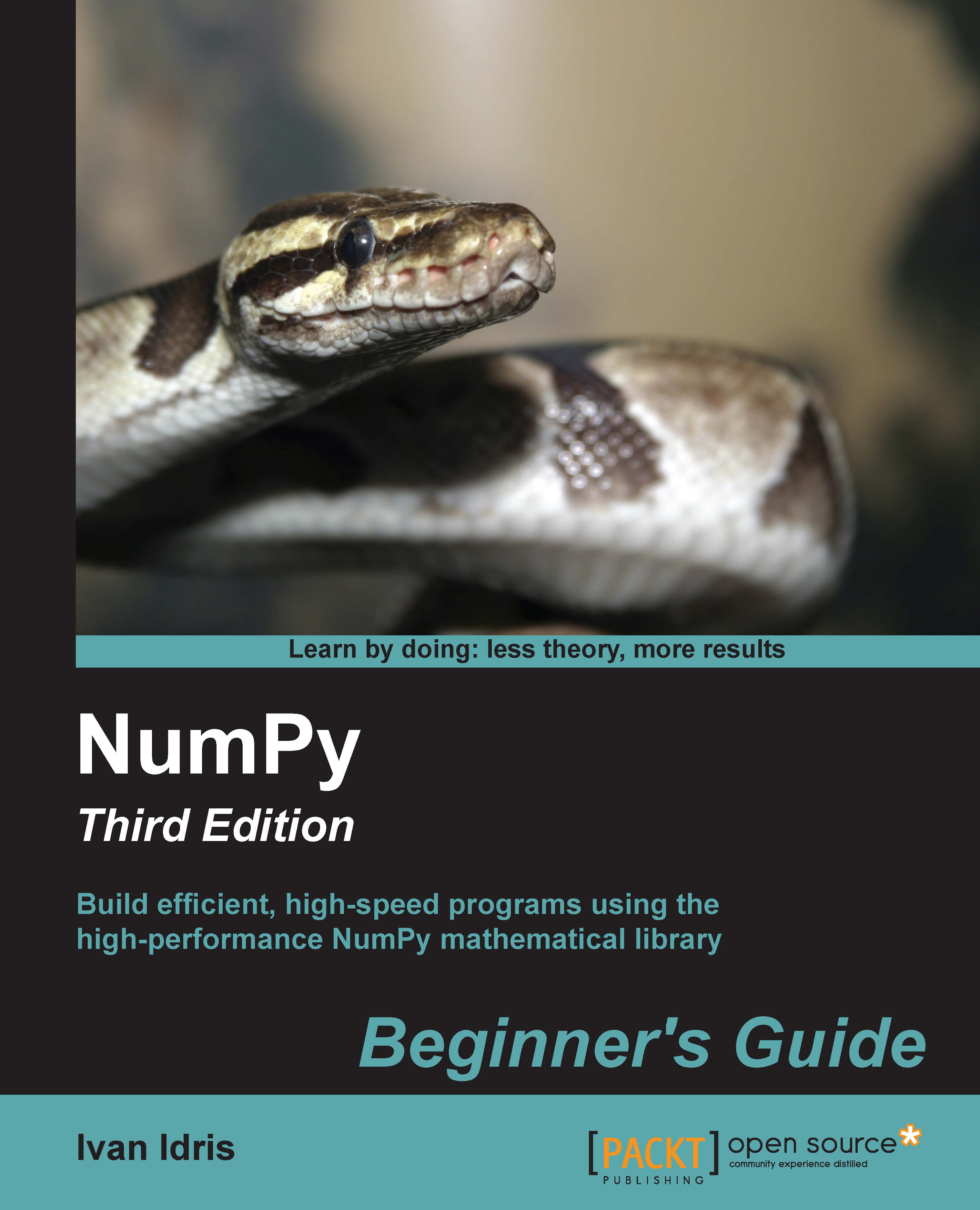
Numpy Beginner's Guide (Update)

Numpy Beginner's Guide (Update): Build efficient, high-speed programs using the high-performance NumPy mathematical library

Arrow left icon
Profile Icon Ivan Idris
Arrow right icon
zł197.99
Full star icon Full star icon Empty star icon Empty star icon Empty star icon 2 (1 Ratings)
Paperback Jun 2015 348 pages 1st Edition
eBook
zł59.99 zł158.99
Paperback
zł197.99
Subscription
Free Trial
Arrow left icon
Profile Icon Ivan Idris
Arrow right icon
zł197.99
Full star icon Full star icon Empty star icon Empty star icon Empty star icon 2 (1 Ratings)
Paperback Jun 2015 348 pages 1st Edition
eBook
zł59.99 zł158.99
Paperback
zł197.99
Subscription
Free Trial
eBook
zł59.99 zł158.99
Paperback
zł197.99
Subscription
Free Trial

What do you get with Print?

Product feature icon Instant access to your digital eBook copy whilst your Print order is Shipped
Product feature icon Paperback book shipped to your preferred address
Product feature icon Download this book in EPUB and PDF formats
Product feature icon Access this title in our online reader with advanced features
Product feature icon DRM FREE - Read whenever, wherever and however you want
OR
Modal Close icon
Payment Processing...
tick Completed

Shipping Address

Billing Address

Shipping Methods
Table of content icon View table of contents Preview book icon Preview Book

Numpy Beginner's Guide (Update)

Chapter 1. NumPy Quick Start

Let's get started. We will install NumPy and related software on different operating systems and have a look at some simple code that uses NumPy. This chapter briefly introduces the IPython interactive shell. SciPy is closely related to NumPy, so you will see the SciPy name appearing here and there. At the end of this chapter, you will find pointers on how to find additional information online if you get stuck or are uncertain about the best way to solve problems.

In this chapter, you will cover the following topics:

  • Install Python, SciPy, matplotlib, IPython, and NumPy on Windows, Linux, and Macintosh
  • Do a short refresher of Python
  • Write simple NumPy code
  • Get to know IPython
  • Browse online documentation and resources

Python

NumPy is based on Python, so you need to have Python installed. On some operating systems, Python is already installed. However, you need to check whether the Python version corresponds with the NumPy version you want to install. There are many implementations of Python, including commercial implementations and distributions. In this book, we focus on the standard CPython implementation, which is guaranteed to be compatible with NumPy.

Time for action – installing Python on different operating systems

NumPy has binary installers for Windows, various Linux distributions, and Mac OS X at http://sourceforge.net/projects/numpy/files/. There is also a source distribution, if you prefer that. You need to have Python 2.4.x or above installed on your system. We will go through the various steps required to install Python on the following operating systems:

  • Debian and Ubuntu: Python might already be installed on Debian and Ubuntu, but the development headers are usually not. On Debian and Ubuntu, install the python and python-dev packages with the following commands:
    $ [sudo] apt-get install python
    $ [sudo] apt-get install python-dev
    
  • Windows: The Windows Python installer is available at https://www.python.org/downloads/. On this website, we can also find installers for Mac OS X and source archives for Linux, UNIX, and Mac OS X.
  • Mac: Python comes preinstalled on Mac OS X. We can also get Python through MacPorts, Fink, Homebrew, or similar projects.

    Install, for instance, the Python 2.7 port by running the following command:

    $ [sudo] port install python27
    

    Linear Algebra PACKage (LAPACK) does not need to be present but, if it is, NumPy will detect it and use it during the installation phase. It is recommended that you install LAPACK for serious numerical analysis as it has useful numerical linear algebra functionality.

What just happened?

We installed Python on Debian, Ubuntu, Windows, and the Mac OS X.

Note

You can download the example code files for all the Packt books you have purchased from your account at https://www.packtpub.com/. If you purchased this book elsewhere, you can visit https://www.packtpub.com/books/content/support and register to have the files e-mailed directly to you.

The Python help system

Before we start the NumPy introduction, let's take a brief tour of the Python help system, in case you have forgotten how it works or are not very familiar with it. The Python help system allows you to look up documentation from the interactive Python shell. A shell is an interactive program, which accepts commands and executes them for you.

Time for action – using the Python help system

Depending on your operating system, you can access the Python shell with special applications, usually a terminal of some sort.

  1. In such a terminal, type the following command to start a Python shell:
    $ python
    
  2. You will get a short message with the Python version and other information and the following prompt:
    >>>
    

    Type the following in the prompt:

    >>> help()
    

    Another message appears and the prompt changes as follows:

    help>
    
  3. If you type, for instance, keywords as the message says, you get a list of keywords. The topics command gives a list of topics. If you type any of the topic names (such as LISTS) in the prompt, you get additional information about the topic. Typing q quits the information screen. Pressing Ctrl + D together returns you to the normal Python prompt:
    >>>
    

    Pressing Ctrl + D together again ends the Python shell session.

What just happened?

We learned about the Python interactive shell and the Python help system.

Basic arithmetic and variable assignment

In the Time for action – using the Python help system section, we used the Python shell to look up documentation. We can also use Python as a calculator. By the way, this is just a refresher, so if you are completely new to Python, I recommend taking some time to learn the basics. If you put your mind to it, learning basic Python should not take you more than a couple of weeks.

Time for action – using Python as a calculator

We can use Python as a calculator as follows:

  1. In a Python shell, add 2 and 2 as follows:
    >>> 2 + 2
    4
    
  2. Multiply 2 and 2 as follows:
    >>> 2 * 2
    4
    
  3. Divide 2 and 2 as follows:
    >>> 2/2
    1
    
  4. If you have programmed before, you probably know that dividing is a bit tricky since there are different types of dividing. For a calculator, the result is usually adequate, but the following division may not be what you were expecting:
    >>> 3/2
    1
    

    We will discuss what this result is about in several later chapters of this book. Take the cube of 2 as follows:

    >>> 2 ** 3
    8
    

What just happened?

We used the Python shell as a calculator and performed addition, multiplication, division, and exponentiation.

Time for action – assigning values to variables

Assigning values to variables in Python works in a similar way to most programming languages.

  1. For instance, assign the value of 2 to a variable named var as follows:
    >>> var = 2
    >>> var
    2
    
  2. We defined the variable and assigned it a value. In this Python code, the type of the variable is not fixed. We can make the variable in to a list, which is a built-in Python type corresponding to an ordered sequence of values. Assign a list to var as follows:
    >>> var = [2, 'spam', 'eggs']
    >>> var
    [2, 'spam', 'eggs']
    

    We can assign a new value to a list item using its index number (counting starts from 0). Assign a new value to the first list element:

    >>> var
    ['ham', 'spam', 'eggs']
    
  3. We can also swap values easily. Define two variables and swap their values:
    >>> a = 1
    >>> b = 2
    >>> a, b = b, a
    >>> a
    2
    >>> b
    1
    

What just happened?

We assigned values to variables and Python list items. This section is by no means exhaustive; therefore, if you are struggling, please read Appendix B, Additional Online Resources, to find recommended Python tutorials.

The print() function

If you haven't programmed in Python for a while or are a Python novice, you may be confused about the Python 2 versus Python 3 discussions. In a nutshell, the latest version Python 3 is not backward compatible with the older Python 2 because the Python development team felt that some issues were fundamental and therefore warranted a radical change. The Python team has committed to maintain Python 2 until 2020. This may be problematic for the people who still depend on Python 2 in some way. The consequence for the print() function is that we have two types of syntax.

Time for action – printing with the print() function

We can print using the print() function as follows:

  1. The old syntax is as follows:
    >>> print 'Hello'
    Hello
    
  2. The new Python 3 syntax is as follows:
    >>> print('Hello')
    Hello
    

    The parentheses are now mandatory in Python 3. In this book, I try to use the new syntax as much as possible; however, I use Python 2 to be on the safe side. To enforce the syntax, each Python 2 script with print() calls in this book starts with:

    >>> from __future__ import print_function
    
  3. Try to use the old syntax to get the following error message:
    >>> print 'Hello'
      File "<stdin>", line 1
        print 'Hello'
                    ^
    SyntaxError: invalid syntax
    
  4. To print a newline, use the following syntax:
    >>> print()
    
  5. To print multiple items, separate them with commas:
    >>> print(2, 'ham', 'egg')
    2 ham egg
    
  6. By default, Python separates the printed values with spaces and prints output to the screen. You can customize these settings. Read more about this function by typing the following command:
    >>> help(print)
    

    You can exit again by typing q.

What just happened?

We learned about the print() function and its relation to Python 2 and Python 3.

Code comments

Commenting code is a best practice with the goal of making code clearer for yourself and other coders (see https://google-styleguide.googlecode.com/svn/trunk/pyguide.html?showone=Comments#Comments). Usually, companies and other organizations have policies regarding code comment such as comment templates. In this book, I did not comment the code in such a fashion for brevity and because the text in the book should clarify the code.

Time for action – commenting code

The most basic comment starts with a hash sign and continues until the end of the line:

  1. Comment code with this type of comment as follows:
    >>> # Comment from hash to end of line
    
  2. However, if the hash sign is between single or double quotes, then we have a string, which is an ordered sequence of characters:
    >>> astring = '# This is not a comment'
    >>> astring
    '# This is not a comment'
    
  3. We can also comment multiple lines as a block. This is useful if you want to write a more detailed description of the code. Comment multiple lines as follows:
    """
     Chapter 1 of NumPy Beginners Guide.
     Another line of comment.
    """
    

    We refer to this type of comment as triple-quoted for obvious reasons. It also is used to test code. You can read about testing in Chapter 8, Assuring Quality with Testing.

The if statement

The if statement in Python has a bit different syntax to other languages, such as C++ and Java. The most important difference is that indentation matters, which I hope you are aware of.

Time for action – deciding with the if statement

We can use the if statement in the following ways:

  1. Check whether a number is negative as follows:
    >>> if 42 < 0:
    ...     print('Negative')
    ... else:
    ...     print('Not negative')
    ...
    Not negative
    

    In the preceding example, Python decided that 42 is not negative. The else clause is optional. The comparison operators are equivalent to the ones in C++, Java, and similar languages.

  2. Python also has a chained branching logic compound statement for multiple tests similar to the switch statement in C++, Java, and other programming languages. Decide whether a number is negative, 0, or positive as follows:
    >>> a = -42
    >>> if a < 0:
    ...     print('Negative')
    ... elif a == 0:
    ...     print('Zero')
    ... else:
    ...     print('Positive')
    ...
    Negative
    

    This time, Python decided that 42 is negative.

What just happened?

We learned how to do branching logic in Python.

The for loop

Python has a for statement with the same purpose as the equivalent construct in C++, Pascal, Java, and other languages. However, the mechanism of looping is a bit different.

Time for action – repeating instructions with loops

We can use the for loop in the following ways:

  1. Loop over an ordered sequence, such as a list, and print each item as follows:
    >>> food = ['ham', 'egg', 'spam']
    >>> for snack in food:
    ...     print(snack)
    ...
    ham
    egg
    spam
    
  2. And remember that, as always, indentation matters in Python. We loop over a range of values with the built-in range() or xrange() functions. The latter function is slightly more efficient in certain cases. Loop over the numbers 1-9 with a step of 2 as follows:
    >>> for i in range(1, 9, 2):
    ...     print(i)
    ...
    1
    3
    5
    7
    
  3. The start and step parameter of the range() function are optional with default values of 1. We can also prematurely end a loop. Loop over the numbers 0-9 and break out of the loop when you reach 3:
    >>> for i in range(9):
    ...     print(i)
    ...     if i == 3:
    ...     print('Three')
    ...     break
    ...
    0
    1
    2
    3
    Three
    
  4. The loop stopped at 3 and we did not print the higher numbers. Instead of leaving the loop, we can also get out of the current iteration. Print the numbers 0-4, skipping 3 as follows:
    >>> for i in range(5):
    ...     if i == 3:
    ...             print('Three')
    ...             continue
    ...     print(i)
    ...
    0
    1
    2
    Three
    4
    
  5. The last line in the loop was not executed when we reached 3 because of the continue statement. In Python, the for loop can have an else statement attached to it. Add an else clause as follows:
    >>> for i in range(5):
    ...     print(i)
    ... else:
    ...     print(i, 'in else clause')
    ...
    0
    1
    2
    3
    4
    (4, 'in else clause')
    
  6. Python executes the code in the else clause last. Python also has a while loop. I do not use it that much because the for loop is more useful in my opinion.

What just happened?

We learned how to repeat instructions in Python with loops. This section included the break and continue statements, which exit and continue looping.

Python functions

Functions are callable blocks of code. We call functions by the name we give them.

Time for action – defining functions

Let's define the following simple function:

  1. Print Hello and a given name in the following way:
    >>> def print_hello(name):
    ...     print('Hello ' + name)
    ...
    

    Call the function as follows:

    >>> print_hello('Ivan')
    Hello Ivan
    
  2. Some functions do not have arguments, or the arguments have default values. Give the function a default argument value as follows:
    >>> def print_hello(name='Ivan'):
    ...     print('Hello ' + name)
    ...
    >>> print_hello()
    Hello Ivan
    
  3. Usually, we want to return a value. Define a function, which doubles input values as follows:
    >>> def double(number):
    ...     return 2 * number
    ...
    >>> double(3)
    6
    

What just happened?

We learned how to define functions. Functions can have default argument values and return values.

Python modules

A file containing Python code is called a module. A module can import other modules, functions in other modules, and other parts of modules. The filenames of Python modules end with .py. The name of the module is the same as the filename minus the .py suffix.

Time for action – importing modules

Importing modules can be done in the following manner:

  1. If the filename is, for instance, mymodule.py, import it as follows:
    >>> import mymodule
    
  2. The standard Python distribution has a math module. After importing it, list the functions and attributes in the module as follows:
    >>> import math
    >>> dir(math)
    ['__doc__', '__file__', '__name__', '__package__', 'acos', 'acosh', 'asin', 'asinh', 'atan', 'atan2', 'atanh', 'ceil', 'copysign', 'cos', 'cosh', 'degrees', 'e', 'erf', 'erfc', 'exp', 'expm1', 'fabs', 'factorial', 'floor', 'fmod', 'frexp', 'fsum', 'gamma', 'hypot', 'isinf', 'isnan', 'ldexp', 'lgamma', 'log', 'log10', 'log1p', 'modf', 'pi', 'pow', 'radians', 'sin', 'sinh', 'sqrt', 'tan', 'tanh', 'trunc']
    
  3. Call the pow() function in the math module:
    >>> math.pow(2, 3)
    8.0
    

    Notice the dot in the syntax. We can also import a function directly and call it by its short name. Import and call the pow() function as follows:

    >>> from math import pow
    >>> pow(2, 3)
    8.0
    
  4. Python lets us define aliases for imported modules and functions. This is a good time to introduce the import conventions we are going to use for NumPy and a plotting library we will use a lot:
    import numpy as np
    import matplotlib.pyplot as plt

What just happened?

We learned about modules, importing modules, importing functions, calling functions in modules, and the import conventions of this book. This concludes the Python refresher.

NumPy on Windows

Installing NumPy on Windows is straightforward. You only need to download an installer, and a wizard will guide you through the installation steps.

Time for action – installing NumPy, matplotlib, SciPy, and IPython on Windows

Installing NumPy on Windows is necessary but this is, fortunately, a straightforward task that we will cover in detail. It is recommended that you install matplotlib, SciPy, and IPython. However, this is not required to enjoy this book. The actions we will take are as follows:

  1. Download a NumPy installer for Windows from the SourceForge website http://sourceforge.net/projects/numpy/files/.
    Time for action – installing NumPy, matplotlib, SciPy, and IPython on Windows

    Choose the appropriate NumPy version according to your Python version. In the preceding screen shot, we chose numpy-1.9.2-win32-superpack-python2.7.exe.

  2. Open the EXE installer by double-clicking on it as shown in the following screen shot:
    Time for action – installing NumPy, matplotlib, SciPy, and IPython on Windows
  3. Now, we can see a description of NumPy and its features. Click on Next.
  4. If you have Python installed, it should automatically be detected. If it is not detected, your path settings might be wrong. At the end of this chapter, we have listed resources in case you have problems with installing NumPy.
  5. In this example, Python 2.7 was found. Click on Next if Python is found; otherwise, click on Cancel and install Python (NumPy cannot be installed without Python). Click on Next. This is the point of no return. Well, kind of, but it is best to make sure that you are installing to the proper directory and so on and so forth. Now the real installation starts. This may take a while.

    Install SciPy and matplotlib with the Enthought Canopy distribution (https://www.enthought.com/products/canopy/). It might be necessary to put the msvcp71.dll file in your C:\Windows\system32 directory. You can get it from http://www.dll-files.com/dllindex/dll-files.shtml?msvcp71 A Windows IPython installer is available on the IPython website (see http://ipython.org/).

What just happened?

We installed NumPy, SciPy, matplotlib, and IPython on Windows.

NumPy on Linux

Installing NumPy and its related recommended software on Linux depends on the distribution you have. We will discuss how you will install NumPy from the command line, although you can probably use graphical installers; it depends on your distribution (distro). The commands to install matplotlib, SciPy, and IPython are the same—only the package names are different. Installing matplotlib, SciPy, and IPython is recommended, but optional.

Time for action – installing NumPy, matplotlib, SciPy, and IPython on Linux

Most Linux distributions have NumPy packages. We will go through the necessary commands for some of the most popular Linux distros:

  • Installing NumPy on Red Hat: Run the following instructions from the command line:
    $ yum install python-numpy
    
  • Installing NumPy on Mandriva: To install NumPy on Mandriva, run the following command line instruction:
    $ urpmi python-numpy
    
  • Installing NumPy on Gentoo: To install NumPy on Gentoo, run the following command line instruction:
    $ [sudo] emerge numpy
    
  • Installing NumPy on Debian and Ubuntu: On Debian or Ubuntu, type the following on the command line:
    $ [sudo] apt-get install python-numpy
    

    The following table gives an overview of the Linux distributions and the corresponding package names for NumPy, SciPy, matplotlib, and IPython:

    Linux distribution

    NumPy

    SciPy

    matplotlib

    IPython

    Arch Linux

    python-numpy

    python-scipy

    python-matplotlib

    ipython

    Debian

    python-numpy

    python-scipy

    python-matplotlib

    ipython

    Fedora

    numpy

    python-scipy

    python-matplotlib

    ipython

    Gentoo

    dev-python/numpy

    scipy

    matplotlib

    ipython

    OpenSUSE

    python-numpy, python-numpy-devel

    python-scipy

    python-matplotlib

    ipython

    Slackware

    numpy

    scipy

    matplotlib

    ipython

NumPy on Mac OS X

You can install NumPy, matplotlib, and SciPy on the Mac OS X with a GUI installer (not possible for all versions) or from the command line with a port manager such as MacPorts, Homebrew, or Fink, depending on your preference. You can also install using a script from https://github.com/fonnesbeck/ScipySuperpack.

Time for action – installing NumPy, SciPy, matplotlib, and IPython with MacPorts or Fink

Alternatively, we can install NumPy, SciPy, matplotlib, and IPython through the MacPorts route or with Fink. The following installation steps show how to install all these packages:

  • Installing with MacPorts: Type the following command:
    $ [sudo] port install py-numpy py-scipy py-matplotlib py-ipython
    
  • Installing with Fink: Fink also has packages for NumPy—scipy-core-py24, scipy-core-py25, and scipy-core-py26. The SciPy packages are scipy-py24, scipy-py25 and scipy-py26. We can install NumPy and the additional recommended packages, referring to this book on Python 2.7, using the following command:
    $ fink install scipy-core-py27 scipy-py27 matplotlib-py27
    

What just happened?

We installed NumPy and the additional recommended software on Mac OS X with MacPorts and Fink.

Building from source

We can retrieve the source code for NumPy with git as follows:

$ git clone git://github.com/numpy/numpy.git numpy

Alternatively, download the source from http://sourceforge.net/projects/numpy/files/.

Install in /usr/local with the following command:

$ python setup.py build
$ [sudo] python setup.py install --prefix=/usr/local

To build, we need a C compiler such as GCC and the Python header files in the python-dev or python-devel packages.

Arrays

After going through the installation of NumPy, it's time to have a look at NumPy arrays. NumPy arrays are more efficient than Python lists when it comes to numerical operations. NumPy code requires less explicit loops than the equivalent Python code.

Time for action – adding vectors

Imagine that we want to add two vectors called a and b (see https://www.khanacademy.org/science/physics/one-dimensional-motion/displacement-velocity-time/v/introduction-to-vectors-and-scalars). Vector is used here in the mathematical sense meaning a one-dimensional array. We will learn in Chapter 5, Working with Matrices and ufuncs, about specialized NumPy arrays, which represent matrices. Vector a holds the squares of integers 0 to n, for instance, if n is equal to 3, then a is equal to (0,1, 4). Vector b holds the cubes of integers 0 to n, so if n is equal to 3, then b is equal to (0,1, 8). How will you do that using plain Python? After we come up with a solution, we will compare it to the NumPy equivalent.

  1. Adding vectors using pure Python: The following function solves the vector addition problem using pure Python without NumPy:
    def pythonsum(n):
       a = range(n)
       b = range(n)
       c = []
    
       for i in range(len(a)):
           a[i] = i ** 2
           b[i] = i ** 3
           c.append(a[i] + b[i])
    
       return c

    Tip

    Downloading the example code files

    You can download the example code files from your account at http://www.packtpub.com for all the Packt Publishing books you have purchased. If you purchased this book elsewhere, you can visit http://www.packtpub.com/support and register to have the files e-mailed directly to you.

  2. Adding vectors using NumPy: Following is a function that achieves the same result with NumPy:
    def numpysum(n):
      a = np.arange(n) ** 2
      b = np.arange(n) ** 3
      c = a + b
    
      return c

Notice that numpysum() does not need a for loop. Also, we used the arange() function from NumPy that creates a NumPy array for us with integers 0 to n. The arange() function was imported; that is why it is prefixed with numpy (actually, it is customary to abbreviate it via an alias to np).

Now comes the fun part. The preface mentions that NumPy is faster when it comes to array operations. How much faster is NumPy, though? The following program will show us by measuring the elapsed time, in microseconds, for the numpysum() and pythonsum() functions. It also prints the last two elements of the vector sum. Let's check that we get the same answers by using Python and NumPy:

#!/usr/bin/env/python

from __future__ import print_function
import sys
from datetime import datetime
import numpy as np

"""
 Chapter 1 of NumPy Beginners Guide.
 This program demonstrates vector addition the Python way.
 Run from the command line as follows
     
  python vectorsum.py n
 
 where n is an integer that specifies the size of the vectors.

 The first vector to be added contains the squares of 0 up to n.
 The second vector contains the cubes of 0 up to n.
 The program prints the last 2 elements of the sum and the elapsed time.
"""

def numpysum(n):
   a = np.arange(n) ** 2
   b = np.arange(n) ** 3
   c = a + b

   return c

def pythonsum(n):
   a = range(n)
   b = range(n)
   c = []

   for i in range(len(a)):
       a[i] = i ** 2
       b[i] = i ** 3
       c.append(a[i] + b[i])

   return c
   

size = int(sys.argv[1])

start = datetime.now()
c = pythonsum(size)
delta = datetime.now() - start
print("The last 2 elements of the sum", c[-2:])
print("PythonSum elapsed time in microseconds", delta.microseconds)

start = datetime.now()
c = numpysum(size)
delta = datetime.now() - start
print("The last 2 elements of the sum", c[-2:])
print("NumPySum elapsed time in microseconds", delta.microseconds)

The output of the program for 1000, 2000, and 3000 vector elements is as follows:

$ python vectorsum.py 1000
The last 2 elements of the sum [995007996, 998001000]
PythonSum elapsed time in microseconds 707
The last 2 elements of the sum [995007996 998001000]
NumPySum elapsed time in microseconds 171
$ python vectorsum.py 2000
The last 2 elements of the sum [7980015996, 7992002000]
PythonSum elapsed time in microseconds 1420
The last 2 elements of the sum [7980015996 7992002000]
NumPySum elapsed time in microseconds 168
$ python vectorsum.py 4000
The last 2 elements of the sum [63920031996, 63968004000]
PythonSum elapsed time in microseconds 2829
The last 2 elements of the sum [63920031996 63968004000]
NumPySum elapsed time in microseconds 274

What just happened?

Clearly, NumPy is much faster than the equivalent normal Python code. One thing is certain, we get the same results whether we use NumPy or not. However, the result printed differs in representation. Notice that the result from the numpysum() function does not have any commas. How come? Obviously, we are not dealing with a Python list but with a NumPy array. It was mentioned in the Preface that NumPy arrays are specialized data structures for numerical data. We will learn more about NumPy arrays in the next chapter.

Pop quiz – Functioning of the arange() function

Q1. What does arange(5) do?

  1. Creates a Python list of 5 elements with the values 1-5.
  2. Creates a Python list of 5 elements with the values 0-4.
  3. Creates a NumPy array with the values 1-5.
  4. Creates a NumPy array with the values 0-4.
  5. None of the above.

Have a go hero – continue the analysis

The program we used to compare the speed of NumPy and regular Python is not very scientific. We should at least repeat each measurement a couple of times. It will be nice to be able to calculate some statistics such as average times. Also, you might want to show plots of the measurements to friends and colleagues.

Tip

Hints to help can be found in the online documentation and the resources listed at the end of this chapter. NumPy has statistical functions that can calculate averages for you. I recommend using matplotlib to produce plots. Chapter 9, Plotting with matplotlib, gives a quick overview of matplotlib.

IPython – an interactive shell

Scientists and engineers are used to experiment. Scientists created IPython with experimentation in mind. Many view the interactive environment that IPython provides as a direct answer to MATLAB, Mathematica, and Maple. You can find more information, including installation instructions, at http://ipython.org/.

IPython is free, open source, and available for Linux, UNIX, Mac OS X, and Windows. The IPython authors only request that you cite IPython in any scientific work that uses IPython. The following is a list of the basic IPython features:

  • Tab completion
  • History mechanism
  • Inline editing
  • Ability to call external Python scripts with %run
  • Access to system commands
  • Pylab switch
  • Access to Python debugger and profiler

The Pylab switch imports all the SciPy, NumPy, and matplotlib packages. Without this switch, we will have to import every package we need ourselves.

All we need to do is enter the following instruction on the command line:

$ ipython --pylab
IPython 2.4.1 -- An enhanced Interactive Python.
?         -> Introduction and overview of IPython's features.
%quickref -> Quick reference.
help      -> Python's own help system.
object?   -> Details about 'object', use 'object??' for extra details.
Using matplotlib backend: MacOSX

In [1]: quit()

The quit()command or Ctrl + D quits the IPython shell. We may want to be able to go back to our experiments. In IPython, it is easy to save a session for later:

In [1]: %logstart
Activating auto-logging. Current session state plus future input saved.
Filename       : ipython_log.py
Mode           : rotate
Output logging : False
Raw input log  : False
Timestamping   : False
State          : active

Let's say we have the vector addition program that we made in the current directory. Run the script as follows:

In [1]: ls
README        vectorsum.py
In [2]: %run -i vectorsum.py 1000

As you probably remember, 1000 specifies the number of elements in a vector. The -d switch of %run starts an ipdb debugger with c the script is started. n steps through the code. Typing quit at the ipdb prompt exits the debugger:

In [2]: %run -d vectorsum.py 1000
*** Blank or comment
Breakpoint 1 at: /Users/…/vectorsum.py:3

Tip

Enter c at the ipdb> prompt to start your script.

><string>(1)<module>()
ipdb> c
> /Users/…/vectorsum.py(3)<module>()
      2
1---> 3 import sys
      4 from datetime import datetime
ipdb> n
>
/Users/…/vectorsum.py(4)<module>()
1     3 import sys
----> 4 from datetime import datetime
      5 import numpy
ipdb> n
> /Users/…/vectorsum.py(5)<module>()
      4 from datetime import datetime
----> 5 import numpy
      6
ipdb> quit

We can also profile our script by passing the -p option to %run:

In [4]: %run -p vectorsum.py 1000
         1058 function calls (1054 primitive calls) in 0.002 CPU seconds
   Ordered by: internal time
ncalls tottime percall cumtime percall filename:lineno(function)
1 0.001    0.001   0.001    0.001 vectorsum.py:28(pythonsum)
1 0.001    0.001   0.002    0.002 {execfile}
1000 0.000    0.0000.0000.000 {method 'append' of 'list' objects}
1 0.000    0.000    0.002    0.002 vectorsum.py:3(<module>)
1 0.000    0.0000.0000.000 vectorsum.py:21(numpysum)
3    0.000    0.0000.0000.000 {range}
1    0.000    0.0000.0000.000 arrayprint.py:175(_array2string)
3/1    0.000    0.0000.0000.000 arrayprint.py:246(array2string)
2    0.000    0.0000.0000.000 {method 'reduce' of 'numpy.ufunc' objects}
4    0.000    0.0000.0000.000 {built-in method now}
2    0.000    0.0000.0000.000 arrayprint.py:486(_formatInteger)
2    0.000    0.0000.0000.000 {numpy.core.multiarray.arange}
1    0.000    0.0000.0000.000 arrayprint.py:320(_formatArray)
3/1    0.000    0.0000.0000.000 numeric.py:1390(array_str)
1    0.000    0.0000.0000.000 numeric.py:216(asarray)
2    0.000    0.0000.0000.000 arrayprint.py:312(_extendLine)
1    0.000    0.0000.0000.000 fromnumeric.py:1043(ravel)
2    0.000    0.0000.0000.000 arrayprint.py:208(<lambda>)
1    0.000    0.000    0.002    0.002<string>:1(<module>)
11    0.000    0.0000.0000.000 {len}
2    0.000    0.0000.0000.000 {isinstance}
1    0.000    0.0000.0000.000 {reduce}
1    0.000    0.0000.0000.000 {method 'ravel' of 'numpy.ndarray' objects}
4    0.000    0.0000.0000.000 {method 'rstrip' of 'str' objects}
3    0.000    0.0000.0000.000 {issubclass}
2    0.000    0.0000.0000.000 {method 'item' of 'numpy.ndarray' objects}
1    0.000    0.0000.0000.000 {max}
1    0.000    0.0000.0000.000 {method 'disable' of '_lsprof.Profiler' objects}

This gives us a bit more insight in to the workings of our program. In addition, we can now identify performance bottlenecks. The %hist command shows the commands history:

In [2]: a=2+2
In [3]: a
Out[3]: 4
In [4]: %hist
1: _ip.magic("hist ")
2: a=2+2
3: a

I hope you agree that IPython is a really useful tool!

Online resources and help

When we are in IPython's pylab mode, we can open manual pages for NumPy functions with the help command. It is not necessary to know the name of a function. We can type a few characters and then let tab completion do its work. Let's, for instance, browse the available information for the arange() function:

In [2]: help ar<Tab>
Online resources and help
In [2]: help arange

Another option is to put a question mark behind the function name:

In [3]: arange?

The main documentation website for NumPy and SciPy is at http://docs.scipy.org/doc/. Through this web page, we can browse the NumPy reference at http://docs.scipy.org/doc/numpy/reference/, the user guide, and several tutorials.

The popular Stack Overflow software development forum has hundreds of questions tagged numpy. To view them, go to http://stackoverflow.com/questions/tagged/numpy.

If you are really stuck with a problem or you want to be kept informed of NumPy development, you can subscribe to the NumPy discussion mailing list. The e-mail address is . The number of e-mails per day is not too high with almost no spam to speak of. Most importantly, the developers actively involved with NumPy also answer questions asked on the discussion group. The complete list can be found at http://www.scipy.org/scipylib/mailing-lists.html.

For IRC users, there is an IRC channel on irc://irc.freenode.net. The channel is called #scipy, but you can also ask NumPy questions since SciPy users also have knowledge of NumPy, as SciPy is based on NumPy. There are at least 50 members on the SciPy channel at all times.

Summary

In this chapter, we installed NumPy and other recommended software that we will be using in some sections of this book. We got a vector addition program working and convinced ourselves that NumPy has superior performance. You were introduced to the IPython interactive shell. In addition, you explored the available NumPy documentation and online resources.

In the next chapter, you will take a look under the hood and explore some fundamental concepts including arrays and data types.

Left arrow icon Right arrow icon

Description

This book is for the scientists, engineers, programmers, or analysts looking for a high-quality, open source mathematical library. Knowledge of Python is assumed. Also, some affinity, or at least interest, in mathematics and statistics is required. However, I have provided brief explanations and pointers to learning resources.

Who is this book for?

This book is for the scientists, engineers, programmers, or analysts looking for a high-quality, open source mathematical library. Knowledge of Python is assumed. Also, some affinity, or at least interest, in mathematics and statistics is required. However, I have provided brief explanations and pointers to learning resources.

What you will learn

  • Install NumPy, matplotlib, SciPy, and IPython on various operating systems
  • Use NumPy array objects to perform array operations
  • Familiarize yourself with commonly used NumPy functions
  • Use NumPy matrices for matrix algebra
  • Work with the NumPy modules to perform various algebraic operations
  • Test NumPy code with the numpy.testing module
  • Plot simple plots, subplots, histograms, and more with matplotlib
Estimated delivery fee Deliver to Poland

Premium delivery 7 - 10 business days

zł110.95
(Includes tracking information)

Product Details

Country selected
Publication date, Length, Edition, Language, ISBN-13
Publication date : Jun 24, 2015
Length: 348 pages
Edition : 1st
Language : English
ISBN-13 : 9781785281969
Category :
Languages :
Concepts :
Tools :

What do you get with Print?

Product feature icon Instant access to your digital eBook copy whilst your Print order is Shipped
Product feature icon Paperback book shipped to your preferred address
Product feature icon Download this book in EPUB and PDF formats
Product feature icon Access this title in our online reader with advanced features
Product feature icon DRM FREE - Read whenever, wherever and however you want
OR
Modal Close icon
Payment Processing...
tick Completed

Shipping Address

Billing Address

Shipping Methods
Estimated delivery fee Deliver to Poland

Premium delivery 7 - 10 business days

zł110.95
(Includes tracking information)

Product Details

Publication date : Jun 24, 2015
Length: 348 pages
Edition : 1st
Language : English
ISBN-13 : 9781785281969
Category :
Languages :
Concepts :
Tools :

Packt Subscriptions

See our plans and pricing
Modal Close icon
$19.99 billed monthly
Feature tick icon Unlimited access to Packt's library of 7,000+ practical books and videos
Feature tick icon Constantly refreshed with 50+ new titles a month
Feature tick icon Exclusive Early access to books as they're written
Feature tick icon Solve problems while you work with advanced search and reference features
Feature tick icon Offline reading on the mobile app
Feature tick icon Simple pricing, no contract
$199.99 billed annually
Feature tick icon Unlimited access to Packt's library of 7,000+ practical books and videos
Feature tick icon Constantly refreshed with 50+ new titles a month
Feature tick icon Exclusive Early access to books as they're written
Feature tick icon Solve problems while you work with advanced search and reference features
Feature tick icon Offline reading on the mobile app
Feature tick icon Choose a DRM-free eBook or Video every month to keep
Feature tick icon PLUS own as many other DRM-free eBooks or Videos as you like for just zł20 each
Feature tick icon Exclusive print discounts
$279.99 billed in 18 months
Feature tick icon Unlimited access to Packt's library of 7,000+ practical books and videos
Feature tick icon Constantly refreshed with 50+ new titles a month
Feature tick icon Exclusive Early access to books as they're written
Feature tick icon Solve problems while you work with advanced search and reference features
Feature tick icon Offline reading on the mobile app
Feature tick icon Choose a DRM-free eBook or Video every month to keep
Feature tick icon PLUS own as many other DRM-free eBooks or Videos as you like for just zł20 each
Feature tick icon Exclusive print discounts

Frequently bought together


Stars icon
Total 509.97
Learning SciPy for Numerical and Scientific Computing Second Edition
zł133.99
Numpy Beginner's Guide (Update)
zł197.99
Mastering Matplotlib
zł177.99
Total 509.97 Stars icon

Table of Contents

15 Chapters
1. NumPy Quick Start Chevron down icon Chevron up icon
2. Beginning with NumPy Fundamentals Chevron down icon Chevron up icon
3. Getting Familiar with Commonly Used Functions Chevron down icon Chevron up icon
4. Convenience Functions for Your Convenience Chevron down icon Chevron up icon
5. Working with Matrices and ufuncs Chevron down icon Chevron up icon
6. Moving Further with NumPy Modules Chevron down icon Chevron up icon
7. Peeking into Special Routines Chevron down icon Chevron up icon
8. Assuring Quality with Testing Chevron down icon Chevron up icon
9. Plotting with matplotlib Chevron down icon Chevron up icon
10. When NumPy Is Not Enough – SciPy and Beyond Chevron down icon Chevron up icon
11. Playing with Pygame Chevron down icon Chevron up icon
A. Pop Quiz Answers Chevron down icon Chevron up icon
B. Additional Online Resources Chevron down icon Chevron up icon
C. NumPy Functions' References Chevron down icon Chevron up icon
Index Chevron down icon Chevron up icon

Customer reviews

Rating distribution
Full star icon Full star icon Empty star icon Empty star icon Empty star icon 2
(1 Ratings)
5 star 0%
4 star 0%
3 star 0%
2 star 100%
1 star 0%
Alexander Sagel Jan 10, 2017
Full star icon Full star icon Empty star icon Empty star icon Empty star icon 2
it's a helpful guide. however, the code examples are inconsistent in style and overflowing with mistakes. requires a thorough revision
Amazon Verified review Amazon
Get free access to Packt library with over 7500+ books and video courses for 7 days!
Start Free Trial

FAQs

What is the delivery time and cost of print book? Chevron down icon Chevron up icon

Shipping Details

USA:

'

Economy: Delivery to most addresses in the US within 10-15 business days

Premium: Trackable Delivery to most addresses in the US within 3-8 business days

UK:

Economy: Delivery to most addresses in the U.K. within 7-9 business days.
Shipments are not trackable

Premium: Trackable delivery to most addresses in the U.K. within 3-4 business days!
Add one extra business day for deliveries to Northern Ireland and Scottish Highlands and islands

EU:

Premium: Trackable delivery to most EU destinations within 4-9 business days.

Australia:

Economy: Can deliver to P. O. Boxes and private residences.
Trackable service with delivery to addresses in Australia only.
Delivery time ranges from 7-9 business days for VIC and 8-10 business days for Interstate metro
Delivery time is up to 15 business days for remote areas of WA, NT & QLD.

Premium: Delivery to addresses in Australia only
Trackable delivery to most P. O. Boxes and private residences in Australia within 4-5 days based on the distance to a destination following dispatch.

India:

Premium: Delivery to most Indian addresses within 5-6 business days

Rest of the World:

Premium: Countries in the American continent: Trackable delivery to most countries within 4-7 business days

Asia:

Premium: Delivery to most Asian addresses within 5-9 business days

Disclaimer:
All orders received before 5 PM U.K time would start printing from the next business day. So the estimated delivery times start from the next day as well. Orders received after 5 PM U.K time (in our internal systems) on a business day or anytime on the weekend will begin printing the second to next business day. For example, an order placed at 11 AM today will begin printing tomorrow, whereas an order placed at 9 PM tonight will begin printing the day after tomorrow.


Unfortunately, due to several restrictions, we are unable to ship to the following countries:

  1. Afghanistan
  2. American Samoa
  3. Belarus
  4. Brunei Darussalam
  5. Central African Republic
  6. The Democratic Republic of Congo
  7. Eritrea
  8. Guinea-bissau
  9. Iran
  10. Lebanon
  11. Libiya Arab Jamahriya
  12. Somalia
  13. Sudan
  14. Russian Federation
  15. Syrian Arab Republic
  16. Ukraine
  17. Venezuela
What is custom duty/charge? Chevron down icon Chevron up icon

Customs duty are charges levied on goods when they cross international borders. It is a tax that is imposed on imported goods. These duties are charged by special authorities and bodies created by local governments and are meant to protect local industries, economies, and businesses.

Do I have to pay customs charges for the print book order? Chevron down icon Chevron up icon

The orders shipped to the countries that are listed under EU27 will not bear custom charges. They are paid by Packt as part of the order.

List of EU27 countries: www.gov.uk/eu-eea:

A custom duty or localized taxes may be applicable on the shipment and would be charged by the recipient country outside of the EU27 which should be paid by the customer and these duties are not included in the shipping charges been charged on the order.

How do I know my custom duty charges? Chevron down icon Chevron up icon

The amount of duty payable varies greatly depending on the imported goods, the country of origin and several other factors like the total invoice amount or dimensions like weight, and other such criteria applicable in your country.

For example:

  • If you live in Mexico, and the declared value of your ordered items is over $ 50, for you to receive a package, you will have to pay additional import tax of 19% which will be $ 9.50 to the courier service.
  • Whereas if you live in Turkey, and the declared value of your ordered items is over € 22, for you to receive a package, you will have to pay additional import tax of 18% which will be € 3.96 to the courier service.
How can I cancel my order? Chevron down icon Chevron up icon

Cancellation Policy for Published Printed Books:

You can cancel any order within 1 hour of placing the order. Simply contact customercare@packt.com with your order details or payment transaction id. If your order has already started the shipment process, we will do our best to stop it. However, if it is already on the way to you then when you receive it, you can contact us at customercare@packt.com using the returns and refund process.

Please understand that Packt Publishing cannot provide refunds or cancel any order except for the cases described in our Return Policy (i.e. Packt Publishing agrees to replace your printed book because it arrives damaged or material defect in book), Packt Publishing will not accept returns.

What is your returns and refunds policy? Chevron down icon Chevron up icon

Return Policy:

We want you to be happy with your purchase from Packtpub.com. We will not hassle you with returning print books to us. If the print book you receive from us is incorrect, damaged, doesn't work or is unacceptably late, please contact Customer Relations Team on customercare@packt.com with the order number and issue details as explained below:

  1. If you ordered (eBook, Video or Print Book) incorrectly or accidentally, please contact Customer Relations Team on customercare@packt.com within one hour of placing the order and we will replace/refund you the item cost.
  2. Sadly, if your eBook or Video file is faulty or a fault occurs during the eBook or Video being made available to you, i.e. during download then you should contact Customer Relations Team within 14 days of purchase on customercare@packt.com who will be able to resolve this issue for you.
  3. You will have a choice of replacement or refund of the problem items.(damaged, defective or incorrect)
  4. Once Customer Care Team confirms that you will be refunded, you should receive the refund within 10 to 12 working days.
  5. If you are only requesting a refund of one book from a multiple order, then we will refund you the appropriate single item.
  6. Where the items were shipped under a free shipping offer, there will be no shipping costs to refund.

On the off chance your printed book arrives damaged, with book material defect, contact our Customer Relation Team on customercare@packt.com within 14 days of receipt of the book with appropriate evidence of damage and we will work with you to secure a replacement copy, if necessary. Please note that each printed book you order from us is individually made by Packt's professional book-printing partner which is on a print-on-demand basis.

What tax is charged? Chevron down icon Chevron up icon

Currently, no tax is charged on the purchase of any print book (subject to change based on the laws and regulations). A localized VAT fee is charged only to our European and UK customers on eBooks, Video and subscriptions that they buy. GST is charged to Indian customers for eBooks and video purchases.

What payment methods can I use? Chevron down icon Chevron up icon

You can pay with the following card types:

  1. Visa Debit
  2. Visa Credit
  3. MasterCard
  4. PayPal
What is the delivery time and cost of print books? Chevron down icon Chevron up icon

Shipping Details

USA:

'

Economy: Delivery to most addresses in the US within 10-15 business days

Premium: Trackable Delivery to most addresses in the US within 3-8 business days

UK:

Economy: Delivery to most addresses in the U.K. within 7-9 business days.
Shipments are not trackable

Premium: Trackable delivery to most addresses in the U.K. within 3-4 business days!
Add one extra business day for deliveries to Northern Ireland and Scottish Highlands and islands

EU:

Premium: Trackable delivery to most EU destinations within 4-9 business days.

Australia:

Economy: Can deliver to P. O. Boxes and private residences.
Trackable service with delivery to addresses in Australia only.
Delivery time ranges from 7-9 business days for VIC and 8-10 business days for Interstate metro
Delivery time is up to 15 business days for remote areas of WA, NT & QLD.

Premium: Delivery to addresses in Australia only
Trackable delivery to most P. O. Boxes and private residences in Australia within 4-5 days based on the distance to a destination following dispatch.

India:

Premium: Delivery to most Indian addresses within 5-6 business days

Rest of the World:

Premium: Countries in the American continent: Trackable delivery to most countries within 4-7 business days

Asia:

Premium: Delivery to most Asian addresses within 5-9 business days

Disclaimer:
All orders received before 5 PM U.K time would start printing from the next business day. So the estimated delivery times start from the next day as well. Orders received after 5 PM U.K time (in our internal systems) on a business day or anytime on the weekend will begin printing the second to next business day. For example, an order placed at 11 AM today will begin printing tomorrow, whereas an order placed at 9 PM tonight will begin printing the day after tomorrow.


Unfortunately, due to several restrictions, we are unable to ship to the following countries:

  1. Afghanistan
  2. American Samoa
  3. Belarus
  4. Brunei Darussalam
  5. Central African Republic
  6. The Democratic Republic of Congo
  7. Eritrea
  8. Guinea-bissau
  9. Iran
  10. Lebanon
  11. Libiya Arab Jamahriya
  12. Somalia
  13. Sudan
  14. Russian Federation
  15. Syrian Arab Republic
  16. Ukraine
  17. Venezuela