Chapter 2: Data Visualization
Activity 2: Line Plot
Solution:
- Create a list of 6 strings for each month, January through June, and save it as x using:
x = ['January','February','March','April','May','June']
- Create a list of 6 values for 'Items Sold' that starts at 1000 and increases by 200, so the final value is 2000 and save it as y as follows:
y = [1000, 1200, 1400, 1600, 1800, 2000]
- Plot y ('Items Sold') by x ('Month') with a dotted blue line and star markers using the following:
plt.plot(x, y, '*:b')
- Set the x-axis to 'Month' using the following code:
plt.xlabel('Month')
- Set the y-axis to 'Items Sold' as follows:
plt.ylabel('Items Sold')
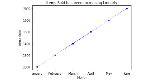
- To set the title to read 'Items Sold has been Increasing Linearly', refer to the following code:
plt.title('Items Sold has been Increasing Linearly')
Check out the following screenshot for the resultant output:

Figure 2.33: Line plot of items sold by month
Activity 3: Bar Plot
Solution:
- Create a list of five strings for x containing the names of NBA franchises with the most titles using the following code:
x = ['Boston Celtics','Los Angeles Lakers', 'Chicago Bulls', 'Golden State Warriors', 'San Antonio Spurs']
- Create a list of five values for y containing values for 'Titles Won' that correspond with the strings in x using the following code:
y = [17, 16, 6, 6, 5]
- Place x and y into a data frame with the column names 'Team' and 'Titles', respectively, as follows:
import pandas as pd
df = pd.DataFrame({'Team': x,
'Titles': y})
- To sort the data frame descending by 'Titles' and save it as df_sorted, refer to the following code:
df_sorted = df.sort_values(by=('Titles'), ascending=False)
Note
If we sort with ascending=True, the plot will have larger values to the right. Since we want the larger values on the left, we will be using ascending=False.
- Make a programmatic title and save it as title by first finding the team with the most titles and saving it as the team_with_most_titles object using the following code:
team_with_most_titles = df_sorted['Team'][0]
- Then, retrieve the number of titles for the team with the most titles using the following code:
most_titles = df_sorted['Titles'][0]
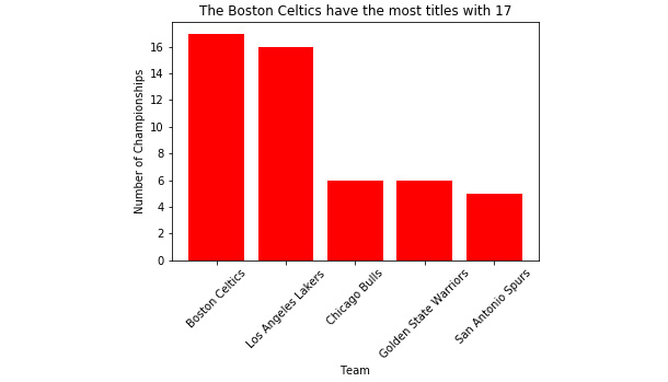
- Lastly, create a string that reads 'The Boston Celtics have the most titles with 17' using the following code:
title = 'The {} have the most titles with {}'.format(team_with_most_titles, most_titles)
- Use a bar graph to plot the number of titles by team using the following code:
import matplotlib.pyplot as plt
plt.bar(df_sorted['Team'], df_sorted['Titles'], color='red')
- Set the x-axis label to 'Team' using the following:
plt.xlabel('Team')
- Set the y-axis label to 'Number of Championships' using the following:
plt.ylabel('Number of Championships')
- To prevent the x tick labels from overlapping by rotating them 45 degrees, refer to the following code:
plt.xticks(rotation=45)
- Set the title of the plot to the programmatic title object we created as follows:
plt.title(title)
- Save the plot to our current working directory as 'Titles_by_Team.png' using the following code:
plt.savefig('Titles_by_Team)
- Print the plot using plt.show(). To understand this better, check out the following output screenshot:

Figure 2.34: The bar plot of the number of titles held by an NBA team
Note
When we print the plot to the console using plt.show(), it appears as intended; however, when we open the file we created titled 'Titles_by_Team.png', we see that it crops the x tick labels.
The following figure displays the bar plot with the cropped x tick labels.

Figure 2.35: 'Titles_by_Team.png' with x tick labels cropped
- To fix the cropping issue, add bbox_inches='tight' as an argument inside of plt.savefig() as follows:
plt.savefig('Titles_by_Team', bbox_inches='tight')
- Now, when we open the saved 'Titles_by_Team.png' file from our working directory, we see that the x tick labels are not cropped.
Check out the following output for the final result:

Figure 2.36: 'Titles_by_Team.png' without cropped x tick labels
Activity 4: Multiple Plot Types Using Subplots
Solution:
- Import the 'Items_Sold_by_Week.csv' file and save it as the Items_by_Week data frame object using the following code:
import pandas as pd
Items_by_Week = pd.read_csv('Items_Sold_by_Week.csv')
- Import the 'Weight_by_Height.csv' file and save it as the Weight_by_Height data frame object as follows:
Weight_by_Height = pd.read_csv('Weight_by_Height.csv')
- Generate an array of 100 normally distributed numbers to use as data for the histogram and box-and-whisker plots and save it as y using the following code:
y = np.random.normal(loc=0, scale=0.1, size=100)
- To generate a figure with six subplots organized in three rows and two columns that do not overlap refer to the following code:
import matplotlib.pyplot as plt
fig, axes = plt.subplots(nrows=3, ncols=2)
plt.tight_layout()
- Set the respective axes' titles to match those in Figure 2.32 using the following code:
axes[0,0].set_title('Line')
axes[0,1].set_title('Bar')
axes[1,0].set_title('Horizontal Bar')
axes[1,1].set_title('Histogram')
axes[2,0].set_title('Scatter')
axes[2,1].set_title('Box-and-Whisker')

Figure 2.37: Titled, non-overlapping empty subplots
- On the 'Line', 'Bar', and 'Horizontal Bar' axes, plot 'Items_Sold' by 'Week' from 'Items_by_Week' using:
axes[0,0].plot(Items_by_Week['Week'], Items_by_Week['Items_Sold'])
axes[0,1].bar(Items_by_Week['Week'], Items_by_Week['Items_Sold'])
axes[1,0].barh(Items_by_Week['Week'], Items_by_Week['Items_Sold'])
See the resultant output in the following figure:

Figure 2.38: Line, bar, and horizontal bar plots added
- On the 'Histogram' and 'Box-and-Whisker' axes, plot the array of 100 normally distributed numbers using the following code:
axes[1,1].hist(y, bins=20)axes[2,1].boxplot(y)
The resultant output is displayed here:

Figure 2.39: The histogram and box-and-whisker added
- Plot 'Weight' by 'Height' on the 'Scatterplot' axes from the 'Weight_by_Height' data frame using the following code:
axes[2,0].scatter(Weight_by_Height['Height'], Weight_by_Height['Weight'])
See the figure here for the resultant output:

Figure 2.40: Scatterplot added
- Label the x- and y-axis for each subplot using axes[row, column].set_xlabel('X-Axis Label') and axes[row, column].set_ylabel('Y-Axis Label'), respectively.
See the figure here for the resultant output:

Figure 2.41: X and y axes have been labeled
- Increase the size of the figure with the figsize argument in the subplots function as follows:
fig, axes = plt.subplots(nrows=3, ncols=2, figsize=(8,8))
- Save the figure to the current working directory as 'Six_Subplots' using the following code:
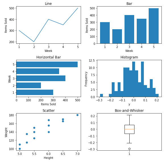
fig.savefig('Six_Subplots')
The following figure displays the 'Six_Subplots.png' file:


