Understanding the basic concepts of pandas
This section will take you through a quick tour of the fundamental concepts of pandas. You will use Jupyter Notebooks to run the code snippets in this book. In the Preface, you learned how to install Anaconda and the required libraries. If you created and installed a separate virtual environment (and kernel) for this book, as shown in the Preface, you'll need to open the Jupyter Notebook, click New in the top-right corner of the Jupyter Notebook navigator, and select the Pandas_Workshop kernel:

Figure 1.1 – Selecting the Pandas_Workshop kernel
A new untitled Jupyter notebook will open that should look something like this:

Figure 1.2 – Jupyter Notebook interface
Installing the conda environment will have also installed pandas. All you need to do now is import the library. You can do so by typing or pasting the following command in a fresh notebook cell:
import pandas as pd
Press the Shift + Enter keyboard shortcut (or click the Run button in the toolbar) to execute the command you just entered:

Figure 1.3 – Importing the pandas library
If you don't see any errors, this means that the library was imported successfully. In the preceding code, the import statement provides all the functionalities of pandas for you to work with. The term pd is a commonly used alias for referring to pandas. You can use any other alias, but pd is used the most.
Now that pandas has been imported, you are ready to roll. Before you start getting your hands dirty and learning about the library in more depth, it is worth taking a quick look at some of the key components and functionalities that pandas offers. At this stage, you don't need to know the details of how they work as you'll be learning about them as you progress through this book.
The Series object
To learn about data wrangling with pandas, you'll need to start from the very beginning, and that is with one-dimensional data. In pandas, one-dimensional data is represented as Series objects. Series objects are initialized using the pd.Series() constructor.
The following code shows how the pd.Series() constructor is used to create a new Series called ser1. Then, simply calling the new Series by its assigned name will display its contents:
Note
If you're running the following code example in a new Jupyter notebook, don't forget to run the import statement shown in the previous section. You'll need to import the pandas library, in the same manner, every time you create a fresh Jupyter notebook.
# Creating a Series
ser1 = pd.Series([10,20,30,40])
# Displaying the Series
ser1
Running the preceding code in a fresh Jupyter notebook cell will produce the following output:

Figure 1.4 – Series object
From the output, you can see that the one-dimensional list is represented as a Series. The numbers to the left of the Series (0, 1, 2, 3) are its indices.
You can represent different types of data in a Series. For example, consider the following snippet:
ser2 = pd.Series([[10, 20],\
[30, 40.5,'series'],\
[50, 55],\
{'Name':'Tess','Org':'Packt'}])
ser2
Running this snippet will result in the following output:

Figure 1.5 – Series output
In the preceding example, a Series was created with multiple data types. You can see that there are lists with numeric and text data (lines 0, 1, and 2) along with a dictionary (line 3). From the output, you can see how these varied data types are represented neatly.
Series help you deal with one-dimensional data. But what about multi-dimensional data? That's where DataFrames come in handy. In the next section, we'll provide a quick overview of DataFrames, one of the most used data structures in pandas.
The DataFrame object
One of the basic building blocks of pandas is the DataFrame structure. A DataFrame is a two-dimensional representation of data in rows and columns, which can be initialized in pandas using the DataFrame() constructor. In the following code, a simple list object is being converted into a one-dimensional DataFrame:
# Create a DataFrame using the constructor
df = pd.DataFrame([30,50,20])
# Display the DataFrame
df
You should get the following output:

Figure 1.6 – DataFrame for list data
This is the simplest representation of a DataFrame. In the preceding code, a list of three elements was converted into a DataFrame using the DataFrame() constructor. The shape of a DataFrame can be visualized using the df.shape() command, as follows:
df.shape
The output will be as follows:
(3, 1)
The output is a DataFrame with a shape of (3,1). Here, the first element (3) is the number of rows, while the second (1) is the number of columns.
If you look at the DataFrame in Figure 1.6, you will see 0 at the top of the column. This is the default name that will be assigned to the column when the DataFrame is created. You can also see the numbers 0, 1, and 2 along the rows. These are called indices.
To display the column names of the DataFrame, you can use the following command:
df.columns
This will result in the following output:
RangeIndex(start=0, stop=1, step=1)
The output shows that it is a range of indices starting at 0 and stopping at 1 with a step size of 1. So, in effect, there is just one column with the name 0. You can also display the names of the indices for the rows using the following command:
df.index
You will see the following output:
RangeIndex(start=0, stop=3, step=1)
As you can see, the indices start from 0 and end at 3 with a step value of 1. This will give the indices 0, 1, and 2.
There are many instances where you would want to use the column names and row indices for further processing. For such purposes, you can convert them into a list using the list() command. The following snippet converts the column names and row indices into lists and then prints those values:
print("These are the names of the columns",list(df.columns))
print("These are the row indices",list(df.index))
You should get the following output:
These are the names of the columns [0]
These are the row indices [0, 1, 2]
From the output, you can see that the column names and the row indices are represented as a list.
You can also rename the columns and row indices by assigning them to any list of values. The command for renaming a column is df.columns, as shown in the following snippet:
# Renaming the columns
df.columns = ['V1']
df
You should see the following output:

Figure 1.7 – Renamed column
Here, you can see that the column has been renamed V1. The command for renaming an index is df.index, as shown in the following snippet:
# Renaming the indices
df.index = ['R1','R2','R3']
df
Running the preceding snippet produces the following output:

Figure 1.8 – Renamed indices
These were examples of DataFrames with just one column. But what if you need to create a DataFrame that contains multiple columns from the list data? This can easily be achieved using a nested list of lists, as follows:
# Creating DataFrame with multiple columns
df1 = pd.DataFrame([[10,15,20],[100,200,300]])
print("Shape of new data frame",df1.shape)
df1
You should get the following output:

Figure 1.9 – Multi-dimensional DataFrame
From the new output, you can see that the new DataFrame has two rows and three columns. The first list forms the first row and each of its elements gets mapped to the three columns. The second list becomes the second row.
You can also assign the column names and row names while creating the DataFrame. To do that for the preceding DataFrame, the following command must be executed:
df1 = pd.DataFrame([[10,15,20],[100,200,300]],\
columns=['V1','V2','V3'],\
index=['R1','R2'])
df1
The output will be as follows:

Figure 1.10 – Renamed columns and indices
From the output, you see that the column names (V1, V2, and V3) and index names (R1 and R2) have been initialized with the user-provided values.
These examples have been provided to initiate you into the world of pandas DataFrames. You can do a lot more complex data analysis using DataFrames, as you will see in the upcoming chapters.
Working with local files
Working with pandas entails importing data from different source files and writing back the outputs in different formats. These operations are indispensable processes when working with data. In the following exercise, you will perform some preliminary operations with a CSV file.
First, you need to download a dataset, Student Performance Data, sourced from the UCI Machine Learning library. This dataset details student achievement in secondary education in two Portuguese schools. Some of the key variables of the dataset include student grades, demographic information, and other social and school-related features, such as hours of study time and prior failures.
Note
You can download the dataset (student-por.csv) from this book's GitHub repository at https://github.com/PacktWorkshops/The-Pandas-Workshop/tree/master/Chapter01/Datasets.
The dataset has been sourced from P. Cortez and A. Silva. Using Data Mining to Predict Secondary School Student Performance. In A. Brito and J. Teixeira Eds., Proceedings of 5th Future Business Technology Conference (FUBUTEC 2008) pp. 5-12, Porto, Portugal, April 2008, EUROSIS, ISBN 978-9077381-39-7.
The following is the link to the original dataset: https://archive.ics.uci.edu/ml/datasets/Student+Performance.
Once the dataset has been downloaded locally, you will be able to read data from it and then display that data using DataFrames. In the next section, we'll briefly cover the pseudocode that will help you read the file you just downloaded. Later, in Exercise 1.01 – reading and writing data using pandas, you will implement the pseudocode to read the CSV file's data into a DataFrame.
Reading a CSV file
To read a CSV file, you can use the following command:
pd.read_csv(filename, delimiter)
The first step of importing data is to define the path to the CSV file. In the preceding code example, the path is defined separately and stored in a variable called filename. Then, this variable is called inside the pd.read_csv() constructor. Alternatively, you can also provide the path directly inside the constructor; for example, 'Datasets/student-por.csv'.
The second parameter, which is the delimiter, specifies how different columns of data are separated within the file. If you open the student-por.csv file in a program such as Excel, you will notice that all the columns in this file are separated using just semicolons (;), as shown in the following screenshot. Therefore, in this case, the delimiter would be a semicolon (;). In the pd.read_csv() constructor, you can represent this as delimiter=';':

Figure 1.11 – Snapshot of the source CSV
Displaying a snapshot of the data
After reading the data from external sources, it is important to ensure that it is loaded correctly. When you have a dataset that contains thousands of rows, it's not a good idea to print out all the rows. In such cases, you can get a snapshot of the dataset by printing only the first few rows. This is where the head() and tail() functions come in handy.
To see the first few rows of the data, you can use the df.head() command, where df is the name of the DataFrame. Similarly, to see the last few rows, you can use the df.tail() command. In both these cases, the first (or last) five rows will be displayed by default. If you want to see more (or fewer) rows, you can specify the number as an argument in the head() or tail() functions. For example, to see the first 10 rows, you can use the df.head(10) function. To see the last seven rows, you can use the df.tail(7) function.
Writing data to a file
There are many instances where you need to write data to a file and store it in a disk for future use. In the next exercise, you will be writing data to a CSV file. You will use the df.to_csv(outpath) command to write data to the file. Here, df is the name of the DataFrame and the outpath parameter is the path where the data must be written.
With that, it is time to put everything we've covered so far into action. The exercise that follows will help you do just that.
Exercise 1.01 – reading and writing data using pandas
In this exercise, you will be working with the student performance dataset you downloaded earlier. The goal of this exercise is to read the data in that file into a DataFrame, display the top rows of the data, and then store a small sample of this data in a new file.
Note
If you haven't downloaded the file yet, the student-por.csv file can be downloaded from https://github.com/PacktWorkshops/The-Pandas-Workshop/tree/master/Chapter01/Datasets.
The following steps will help you complete this exercise:
- Open a new Jupyter notebook and select the Pandas_Workshop kernel, as shown in the following screenshot:
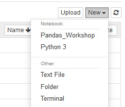
Figure 1.12 – Selecting the Pandas_Workshop kernel
- Import the
pandaslibrary by typing or pasting the following command in a fresh Jupyter Notebook cell. Press the Shift + Enter keyboard combination to run the command:import pandas as pd
- Define the path to the downloaded file. Specify the path where the data has been downloaded in a variable named
filename:filename = '../Datasets/student-por.csv'
Note
The preceding code assumes that the CSV file is stored in a directory called
datasetsoutside of the directory where the code is run. Based on where you have downloaded and stored the file, you'll have to make changes to the pathname (highlighted in the preceding line of code). If your file is stored in the same directory as your Jupyter notebook, thefilenamevariable would just contain thestudent-por.csvvalue. - Read the file using the
pd.read_csv()function, as follows:studentData = pd.read_csv(filename, delimiter=';')
Here, you have stored the data in a variable called studentData, which will be the name of your DataFrame.
- Display the first five rows of data, as follows:
studentData.head()
You should get the following output:

Figure 1.13 – The first five rows of the studentData DataFrame
After displaying the top five rows of data, you can see that the data is spread across 33 columns.
- Make a new DataFrame consisting of only the first five rows. Take the first five rows of the data and then store it in another variable called
studentSmall:studentSmall = studentData.head()
You'll be writing this small dataset to a new file in the subsequent steps.
- Define the output path of the file to write to using the following command:
outpath = '../Datasets/studentSmall.csv'
Note
The path provided in the preceding command (highlighted) specifies the output path and the filename. You can change these values based on where you want the output files to be saved.
- Run the following command to create a CSV file called
studentSmall.csvin the output path you have specified:# Write the data to disk studentSmall.to_csv(outpath)
- Using File Explorer (on Windows), Finder (on macOS), or even the command line, you can check whether the file has been saved to the
Datasetsfolder (or whichever folder you chose). Upon opening the newly saved file in Excel (or any other compatible program), you'll notice that its contents are the same as the DataFrame you created in Step 6:

Figure 1.14 – Contents of the studentSmall.csv file
In this exercise, you read data from a CSV file, created a small sample of the dataset, and wrote it to disk. This exercise was meant to demonstrate one facet of pandas' input/output capabilities. pandas can also read and write data in multiple formats, such as Excel files, JSON files, and HTML, to name a few. We will explore how to input and output different data sources in more detail in Chapter 3, Data I/O.
Data types in pandas
pandas supports different data types, such as int64, float64, date, time, and Boolean. There will be innumerable instances in your data analysis life cycle where you will need to convert data from one type into the other. In such instances, it is imperative to understand these different data types. The operations you'll learn about in this section will help you understand these types.
For this section, you'll need to continue with the same Jupyter notebook that you used to implement Exercise 1.01 – reading and writing data using pandas, as the same dataset will be used in this section too.
The first aspect to know when working with any data is the different data types involved. This can be done using the df.dtypes method, where df is the name of the DataFrame. If you tried the same command on the studentData DataFrame you created in Step 4 of the first exercise, the command would look something like this:
studentData.dtypes
The following is a small part of the output you will get:

Figure 1.15 – Data types in the studentData DataFrame
From the output, you can see that the DataFrame has two data types – object and int64. The object data type refers to string/text data or a combination of numeric and non-numeric data. The int64 data type pertains to integer values.
Additionally, you can get information about the data types by using the df.info() method:
studentData.info()
The following is a small part of the output you will get:

Figure 1.16 – Information about the data types
Here, you can see that this method provides information about the number of null/non-null values, along with the number of rows, in the dataset. In this case, all 649 rows contain non-null data.
pandas also allows you to easily convert data from one type into another using the astype() function. Suppose you want to convert one of the int64 data types into float64. You can do this for the Medu feature (in other words, the column), as follows:
# Converting 'Medu' to data type float
studentData['Medu'] = studentData['Medu'].astype('float')
studentData.dtypes
The following is a small part of the output you will get:
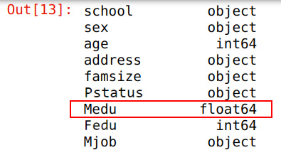
Figure 1.17 – Data type after conversion
When you converted the data type using the astype() function, you had to specify the target data type. Then, you stored the changes in the same variable. The output shows that the int64 data type has changed to float64.
You can display the head of the changed DataFrame and see the changes in the values of the variable by using the following command:
studentData.head()
You should get the following output:

Figure 1.18 – DataFrame after type conversion
From the output, you can see that the values have been converted into float values.
What you have seen so far are only the basic operations for converting data types. There are some interesting transformations you can do on data types, which you will learn about in Chapter 4, Data Types.
In the next section, we'll cover data selection methods. You will need to use the same Jupyter notebook that you've used so far in the next section as well.
Data selection
So far, you have seen operations that let you import data from external files and create data objects such as DataFrames from that imported data. Once a data object such as a DataFrame has been initialized, it is possible to extract relevant data from that data object using some of the intuitive functionalities pandas provides. One such functionality is indexing.
Indexing (also known as subsetting) is a method of extracting a cross-section of data from a DataFrame. First, you will learn how to index some specific columns of data from the studentData DataFrame.
To extract the age column from the DataFrame, you can use the following command:
ageDf = studentData['age']
ageDf
You should see the following output:

Figure 1.19 – The age variable
From the output, you can see how the age column is saved as a separate DataFrame. Similarly, you can subset multiple columns from the original DataFrame, as follows:
# Extracting multiple columns from DataFrame
studentSubset1 = studentData[['age','address','famsize']]
studentSubset1
You should get the following output:
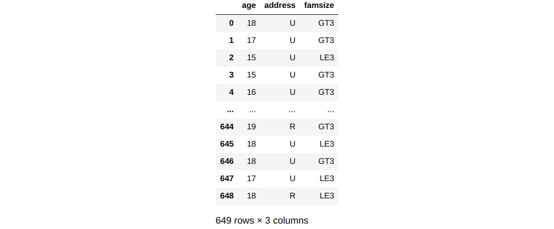
Figure 1.20 – Extracting multiple features
Here, you can see how multiple columns (age, address, and famsize) have been extracted into a new DataFrame. When multiple columns must be subsetted, all of them are represented as a list, as shown in the preceding example.
You can also subset specific rows from a DataFrame, as follows:
studentSubset2 = studentData.loc[:25,['age','address','famsize']]
studentSubset2.shape
You will see the following output for the preceding snippet:
(26, 3)
To subset specific rows, you can use a special operand called .loc(), along with the label indices of the rows you want. In the previous example, the subsetting was done until the 25th row of the dataset. From the output, you can see that the data has 26 rows and that the 25th row is also included in the subsetting.
Subsetting/indexing is a critical part of the data analytics process. pandas has some versatile functions for extracting cross-sections of data. These will be covered in detail in Chapter 5, Data Selection – DataFrames, and Chapter 6, Data Selection – Series.
In the next section, you will look at some data transformation methods. Again, you will continue using the same Jupyter notebook you've used so far.
Data transformation
Once you have created a DataFrame from source files or subset data to a new form, further transformations, such as cleaning up variables or treating for missing data, will be required. There may also be instances where you must group the data based on some variables to analyze data from a different perspective. This section will cover examples of some useful methods for data transformation.
One scenario where you may need to group data would be when you want to verify the number of students under each category of family size. In the family size feature, there are two categories: GT3 (greater than three members) and LE3 (less than three members). Let's say you want to know how many students there are under each of these categories.
To do that, you must take the family size column (famsize), identify all the unique family sizes within this column, and then find the number of students under each size category. This can be achieved by using two simple functions called groupby and agg:
studentData.groupby(['famsize'])['famsize'].agg('count')

Figure 1.21 – Data aggregation
Here, you grouped the DataFrame by the famsize variable using the groupby function. After this, you used the count aggregate function to count the number of records under each famsize category. From the output, you can see that there are two categories of family size, LE3 and GT3, and that the majority fall under the GT3 category.
As you can see from this example, all the different steps listed earlier can be achieved using a single line of code. Just like these, different types of transformations are possible with pandas.
In the next section, you will learn about some data visualization methods.
Data visualization
There is an old saying: "A picture is worth a thousand words." This adage has a profound place in data analytics. Data analytics would be incomplete and would look hollow without proper visualization. matplotlib is a popular library for data visualization that works quite well with pandas. In this section, you will create some simple visualizations of the aggregated data you created in the previous section.
Consider that you want to visualize the number of students under each family size category:
aggData = studentData.groupby(['famsize'])['famsize'].agg('count')
aggData
You should get the following output:

Figure 1.22 – Data aggregation
Here, the groupby function is used to aggregate the family size (famsize) column.
Before plotting this data, you need to create the x- and y-axis values. To define them, with the help of unique indices of grouped data, you can add the following code:
x = list(aggData.index)
x
You will see the following output:
['GT3', 'LE3']
In the preceding code, you took the index values of the aggregated data as the x-axis values. The next step is to create the y-axis values:
y = aggData.values
y
You should see the following output:
array([457, 192], dtype=int64)
The aggregated values for each category in the family size column are on the y axis.
Having obtained the x- and y-axis values, you can plot them using matplotlib, as follows:
import matplotlib.pyplot as plt
%matplotlib inline
plt.style.use('ggplot')
# Plotting the data
plt.bar(x, y, color='gray')
plt.xlabel("Family Sizes")
plt.ylabel("Count of Students ")
plt.title("Distribution of students against family sizes")
plt.show()
Note
In the preceding snippet, the gray value for the color attribute (emboldened) was used to generate graphs in grayscale. You can use other colors, such as darkgreen or maroon, as values of color parameters to get colored graphs.
You will get the following output:
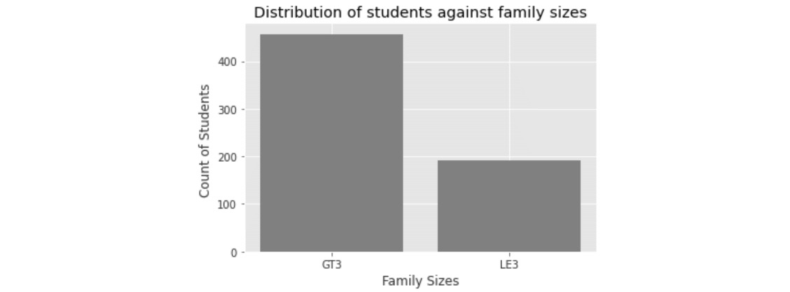
Figure 1.23 – Plots of family size
In the preceding snippet, the first line imports the matplotlib package. The % inline command ensures that the visualization appears in a cell in the same notebook rather than having it pop up as a separate window. This plotting uses a styling called ggplot, which is a popular plotting library that's used in R.
The plt.bar() method plots the data in the form of a bar chart. Inside this method, you can define the x-axis and y-axis values and also define the color. The rest of the lines in the snippet define the labels of the x and y axes, along with the title of the chart. Finally, the plot is displayed with the plt.show() line.
Matplotlib works well with pandas to create impressive visualizations. This topic will be explored in detail in Chapter 8, Data Visualization.
In the next section, you will see how pandas provides utilities to manipulate date objects.
Time series data
Time series data can be seen everywhere in your day-to-day life. Data emitted from social media, sensor data, browsing patterns from e-commerce sites, and log stream data from data centers are all examples of time series data. Preprocessing time series data necessitates performing various transformation operations on time components such as month, year, hours, minutes, and seconds.
In this section, we'll briefly cover some transformation functions with date and time objects. Suppose that you want to convert a string into a date object in pandas. This can be achieved using a handy function called pd.to_datetime():
date = pd.to_datetime('15th of January, 2021')
print(date)
You should get the following output:
2021-01-15 00:00
From the output, you can see that the string object has been converted into a date. Next, suppose you want to calculate the date 25 days from the date you got in the preceding output. To do so, you can run the following code:
# date after 25 days
newdate = date+pd.to_timedelta(25,unit='D')
print(newdate)
You will get the following output:
2021-02-09 00:00:00
As you can see, the pd.to_timedelta() function provides an intuitive way of calculating the date after a prescribed number of days. The unit='D' parameter is used to define that the conversion must be in days.
Next, suppose you want to get all the dates from a start date to a certain period of days. This can be achieved as follows:
# Get all dates within the next 7 days
futureDate = pd.date_range(start=newdate, periods=7, freq='D')
futureDate
You should get the following output:

Figure 1.24 – Date range output
In this example, the date_range() function was used to get a list of all future dates. The start parameter defines the date where you need to start calculating the ranges. The period parameter indicates the number of days it has to calculate from the start date, while freq = 'D' indicates that the unit is in days.
There are many more transformation functions available in pandas for working with time objects. These functions will be covered in greater depth in Chapter 11, Time Series Data.
Code optimization
If datasets get larger or if speed becomes a concern, there are numerous optimization techniques available to increase performance or improve the memory footprint. These range from idiomatic loops over appropriate data types and methods to custom extensions.
One of the many optimization techniques available in pandas is called vectorization. Vectorization is the process of applying an operation over an entire array. pandas has some efficient vectorization processes that enable faster data processing, such as apply and lambda, which will be briefly covered in this section.
As you might know, the apply method is used to apply a function to every element of a Series and the lambda function is a way to create anonymous functions in an operation. Very often, the apply and lambda functions are used in conjunction for efficient implementation.
In the following example, you will learn how to create a new dataset by applying a function to each of the grade variables (G1, G2, G3). The function takes each element of the grade feature and increments it by 5. First, you will only use the apply function; after, you will use the lambda function.
To implement the apply function, you must create a simple function. This function takes an input and adds 5 to it:
# Defining the function
def add5(x):
return x + 5
Now, this function will be used on each element of the grade feature using the apply function:
# Using apply method
df = studentData[['G1','G2','G3']].apply(add5)
df.head()
You should get the following output:

Figure 1.25 – Output after using the apply function
This can also be achieved without defining a separate function using the lambda method, as follows:
df = studentData[['G1','G2','G3']].apply(lambda x:x+5)
df.head()
You should get the following output:

Figure 1.26 – Output after using the lambda function
Here, the lambda() method lets you execute the operation in just one line of code. There is no need to create a separate function.
The example you have implemented is a relatively simple one in terms of using vectorization. Many more complex tasks can be optimized using vectorization. Moreover, vectorization is one of the many methods of code optimization that are used in pandas. You will learn more about it in Chapter 12, Code Optimization.
So far, you have got a bird's-eye view of the topics that will be covered in this book. All these topics will be dealt with in more depth. Now, it's time to apply the concepts you've learned so far in a couple of exercises. Then, you can test what you've learned by completing this chapter's activity.
Utility functions
In the exercises that follow, you will be using some utility functions. These are as follows:
- Generating random numbers using
random():
There will be many instances in the data analytics life cycle where you will have to generate data randomly. numpy is a library in Python that contains some good functions for generating random numbers. Consider the following example:
# Generating random numbers
import numpy as np
np.random.normal(2.0, 1, 10)
You should get the following output:

Figure 1.27 – Output of using the random function
In this example, you imported the numpy library and then used the np.random.normal() function to generate 10 numbers from a normal distribution with a mean of 2 and a standard deviation of 1. You will be utilizing this function in the upcoming exercises.
- Concatenating multiple data series using
pd.concat():
Another commonly used function is concat, which is used to concatenate multiple data elements together. This can be seen in the following code:
# Concatenating three series
pd.concat([ser1,ser2,ser3], axis=1)
In this example, you are concatenating three series using the pd.concat() function. The axis=1 parameter specifies that the concatenation is to be done along the columns. Alternatively, axis=0 means concatenation along the rows, as shown in the following screenshot:
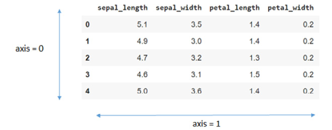
Figure 1.28 – Representation of the axis argument
- The
df.sum,df.mean, anddivmodnumeric functions:
You will be using these numeric functions in the upcoming exercises. The first one, df.sum, is used to calculate the sum of the values in a DataFrame. If you want to find the sum of the DataFrame elements in the columns, you can use the axis=0 argument; for example, df.sum(axis=0).
For example, for the DataFrame shown in the preceding screenshot, df.sum(axis=0) would give you the following output:

Figure 1.29 – Example of axis summation
Defining axis=1, on the other hand, sums up the values along the rows. For example, for the same dataset, df.sum(axis=1) will give the following output:

Figure 1.30 – Output of axis summation
Similarly, df.mean calculates the mean values of the data. The direction of calculation can also be defined using the axis parameter. Finally, divmod is used to calculate the quotient and remainder of a division operation.
You will also use two data manipulation methods, apply and applymap, in the upcoming exercises. The first method, apply, can be used for both Series and DataFrame objects. The second method, applymap, can only be used for DataFrames. The output you get after applying these methods depends on the functions that were used inside these methods as arguments.
- The
to_numericandto_numpydata type conversion functions:
Two commonly used data type conversion functions are to_numeric and to_numpy. The first one, to_numeric, is used to change the data type of any data object to the numeric data type. The second function, to_numpy, is used to convert a pandas DataFrame into a numpy array. Both of these functions are used extensively for data manipulation.
- The
df.eq,df.gt, anddf.ltDataFrame comparison functions:
There will be many instances where you will need to compare one DataFrame to another. pandas provides some good comparison functions to do this. Some of the common ones are df.eq, df.gt, and df.lt. The first method displays all the elements of one DataFrame that are equal to the one in the second DataFrame. Similarly, df.gt finds those elements that are greater in one DataFrame, while the df.lt method finds those elements that are less than those in the other one.
- List comprehension:
List comprehension is a syntax that's used in Python to create lists based on existing lists. Using list comprehension helps avoid the use of for loops. For example, suppose you want to extract every letter from the word Pandas. One way to do this is to use a for loop. Consider the following snippet:
# Define an empty list
letters = []
for letter in 'Pandas':
    letters.append(letter)
print(letters)
You should see the following output, as expected:
['P', 'a', 'n', 'd', 'a', 's']
However, using a list comprehension is much easier and more compact, as follows:
letters = [ letter for letter in 'Pandas' ]
print(letters)
Again, you should get the following output:
['P', 'a', 'n', 'd', 'a', 's']
As shown in the preceding example, using a list comprehension has optimized the code into just one line.
- The
df.iloc()data selection method:
The df.loc() method is used to select specific rows of a DataFrame. Similar to this, there is another function, df.iloc(), that selects specific indices of the data. Let's understand this with a simple example.
Let's create a DataFrame, df:
# Create a Data Frame
lst = [['C', 45], ['A', 60],
       ['A', 26], ['C', 57], ['C', 81]]

df = pd.DataFrame(lst, columns =['Product', 'Sales'])
df
You should see the following output:

Figure 1.31 – Creating a DataFrame
Suppose you want to subset the first three rows for the Sales column. Here, you can use the df.loc() method, as follows:
df.loc[:2,'Sales']
Running this snippet should result in the following output:

Figure 1.32 – Selecting the first three rows
In the preceding code, :2 indicates rows up to index 2. The second parameter, Sales, indicates the columns that need to be selected.
If you want to select a particular index in the DataFrame, you can use the df.iloc() method, as shown here:
df.iloc[3]
You should see the following output:

Figure 1.33 – Selecting an index
- Boolean indexing:
Another important concept in pandas is Boolean indexing. Consider the same sales data you created in the previous example:

Figure 1.34 – Sales data
Suppose you want to find out all the Sales values that equal 45. To do this, you can subset the data, as follows:
df['Sales'].eq(45)
Running this will produce the following output:

Figure 1.35 – Finding which Sales values are equal to 45
Here, you get a Boolean output (True or False), depending on whether the row satisfies the condition – that is, the value of Sales is equal to 45. However, if you want the actual row and its value, rather than the Boolean output, you should apply another type of subsetting, as follows:
df[df['Sales'].eq(45)]
With the additional subsetting, you will get the following output:

Figure 1.36 – Finding which row has a Sales value equal to 45
Here, you can see that the first row satisfies the condition. Now that you have learned about the utility functions, it is time to dive into the second exercise.
Exercise 1.02 – basic numerical operations with pandas
Tess is running a training session on pandas for a few apprentice data analysts who will be working with her. As part of their training, they need to generate some data and perform numerical operations on it, such as summation, mean, and modulus operations. The goal of this exercise is to help Tess conduct her training by running and validating all the code she will be using.
To achieve this, you will need to do the following:
- Create DataFrames from the Series objects.
- Find summary statistics of the DataFrame using the mean, sum, and modulus operations.
- Use the
applymap()method along with lambda functions. - Create new features using list comprehension and concatenate them with an existing DataFrame.
- Change the data type to
int64. - Convert the DataFrame into a
numpyarray.
Follow these steps to complete this exercise:
- Open a new Jupyter notebook and select the Pandas_Workshop kernel.
- Import
pandas,numpy, andrandominto your notebook:import pandas as pd import numpy as np import random
- Create three Series by generating some random data points. To do this, start by sampling 100 data points from three different normal distributions. The first one should have a mean of
3.0and a standard deviation of1. The second and third Series should have the mean and standard values at5.0and3and1.0and0.5, respectively. The sampled data must be converted into a pandas Series:# Initialize a random seed np.random.seed(123) # Create three series ser1 = pd.Series(np.random.normal(3.0, 1, 100)) ser2 = pd.Series(np.random.normal(5.0, 3, 100)) ser3 = pd.Series(np.random.normal(1.0, 0.5, 100))
Here, you used the random.seed() method. This method ensures that you get the same results that were mentioned in this example.
- Concatenate all three Series into a DataFrame. Name the columns and display the first few rows of the newly created DataFrame:
Df = pd.concat([ser1,ser2,ser3], axis=1)
# Name the columns
Df.columns=['V1','V2','V3']
# Display the head of the column
Df.head()
You should get the following output:

Figure 1.37 – Concatenating the Series into a DataFrame
- Next, find the sum of the DataFrame along the columns using the
df.sumfunction:Df.sum(axis=0)
You should get the following output:

Figure 1.38 – Result of summation along the columns
- The
axis=0parameter defines the operation across the rows. Here, you can see three mean values corresponding to each of the columns,V1,V2, andV3. Alternatively,axis=1carries out the operation across the columns. Here, you will be able to see 100 values, where there will be one value corresponding to each row. - Calculate the mean of the values across both the columns and rows using the
df.meanfunction:# Find the mean of the columns Df.mean(axis=0)
You will get the following output:

Figure 1.39 – Mean of the columns
Now, find the mean across the rows:
# Find the mean across the rows
Df.mean(axis=1)
You should get the following output:

Figure 1.40 – Mean across the rows
- Next, find the modulus of each column by using the
divmodfunction. Use this function in conjunction with thelambdaandapplyfunctions:# Apply the divmod function to each of the series Df.apply(lambda x: divmod(x,3))
You should get the following output:

Figure 1.41 – Output of the divmod function
From the code, you can see how the apply function applies the divmod function to each of the Series. The divmod function generates the quotients and remainders for each of the values in the Series. The first row corresponds to the quotients, while the second row corresponds to the remainders.
- In the preceding step, when you implemented the
applymethod,divmodwas applied column-wise. So, you can see that the quotients for all the rows under theV1column are aggregated in row0, columnV1, while the remainders for columnV1are aggregated in row1, columnV1. However, if you want to find the quotient and remainder for each cell of the DataFrame, you can do so usingapplymap, as follows:Df.applymap(lambda x: divmod(x,3))
You should get the following output:
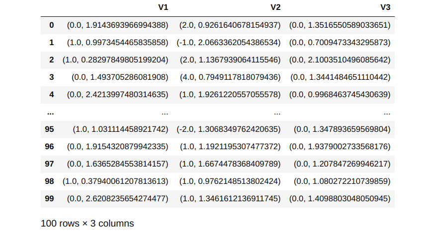
Figure 1.42 – Output after using divmod with applymap
When you use applymap() for the divmod() function in this way, the quotient along with the remainder is generated as a tuple in the output.
- Now, create another character Series and then use the
to_numericfunction to convert the Series into a numeric format. After converting it into a numeric format, concatenate the Series with the existing DataFrame. As a first step, create a list of characters and display its length, as follows:# Create a list of characters list1 = [['20']*10,['35']*15,['40']*10,['10']*25,['15']*40] # Convert them into a single list using list comprehension charlist = [x for sublist in list1 for x in sublist] # Display the output len(charlist)
You should get the following output:
100
In the first line, you created a nested list of character numbers. Then, this nested list was converted into a single list using list comprehension. Finally, the length of the list was displayed, using the len() function, to ensure that there are 100 elements in the list.
- Next, convert the preceding list into a Series object using the
pd.Series()function. Randomly shuffle the list using therandom.shuffle()function before creating the Series:# Randomly shuffle the character list random.seed(123) random.shuffle(charlist) # Convert the list to a series ser4 = pd.Series(charlist) ser4
You should get the following output:
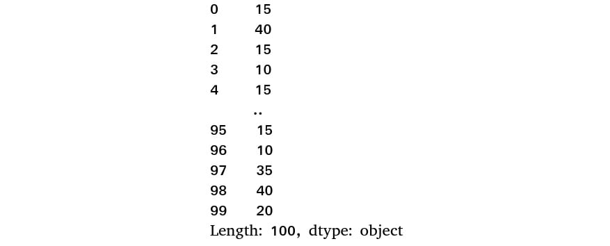
Figure 1.43 – The new Series
Here, you can see that the data type is object, indicating that this is a Series of character data types.
- Now, convert the data type into numeric using the
to_numericfunction:ser4 = pd.to_numeric(ser4) ser4
You will get the following output:

Figure 1.44 – The Series after converting the data type into numeric
Note that the data type has now changed to int64 from object.
- Concatenate the fourth Series that you created in the preceding step, store it in a new DataFrame, and then display its contents by converting it into a
numpyarray:Df = pd.concat([Df,ser4],axis=1) # Renaming the data frame Df.rename(columns={0:'V4'}, inplace=True) # Displaying the data frame Df
You should get the following output:
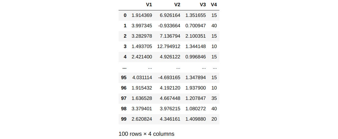
Figure 1.45 – New DataFrame after the addition of a new Series
Here, the inplace=True parameter means that a new DataFrame is created after a new variable has been added.
- Next, convert the DataFrame into a
numpyarray:numpArray = Df.to_numpy()
Now, display the array:
numpArray
You should get the following output. Please note that this has been truncated:
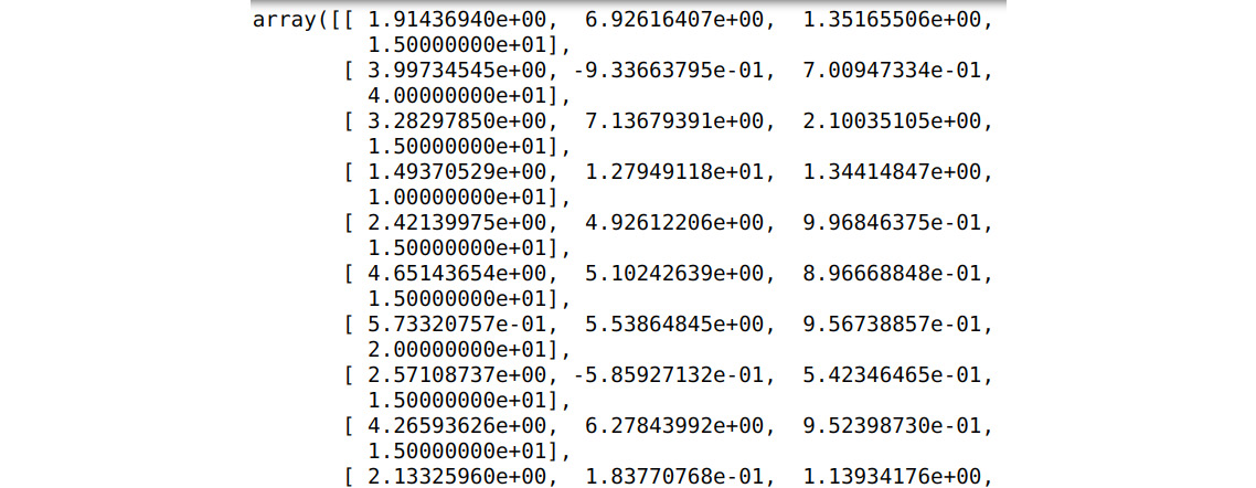
Figure 1.46 – DataFrame converted into a numpy array
Here, you can see that the DataFrame has been converted into a numpy array.
In this exercise, you implemented several numerical functions, such as df.sum, df.mean, and divmod. You also reinforced your understanding of other important functions, such as apply and lambda.
Having learned about some utility functions and applied them in this exercise, you can now move on to the last topic in this chapter. There, you will briefly learn how pandas can be used for building models. You will be using the same Jupyter notebook you've used so far in the next section as well.
Data modeling
A big factor behind the popularity of pandas is its utility in the data science life cycle. pandas has become a tool for most of the data science preprocessing steps, such as data imputation, scaling, and normalization. These are important steps for building machine learning models.
Another important process in the data science life cycle where pandas can be very useful is in creating train and test sets. Training datasets are used to create machine learning models, while test datasets are used to evaluate the performance of the machine learning models that have been built after using the training set. pandas is a go-to tool for creating train and test sets.
Note
If you do not understand the concepts of modeling at this point, that's okay. Just run the code as-is. These concepts will be explained in detail in Chapter 10, Data Modeling.
Consider that a given dataset has been split into train and test sets using pandas. You can use the student dataset you used earlier and split it into two parts, as follows:
# Sampling 80% of data as train data
train=studentData.sample(frac=0.8,random_state=123)
# Rest of the data is taken as test data
test=studentData.drop(train.index)
First, you sampled 80% of the data randomly. The fraction of train data is specified using the frac=0.8 parameter. The data sampling for the train and test sets happens randomly. However, to get the same train and test sets, you can use a parameter called random_state and define a seed number for this (in this case, 123). Every time you use the same seed number, you will get a similar dataset. You can change the dataset by changing the seed number. This process is called reproducing results using a pseudorandom number. The random_state=123 parameter has been set so that you also get results that are similar to the ones shown here.
Once the training data has been sampled, the next task is to drop those samples from the original dataset to get the test data. Using the following code, you can look at the shapes of the train and test datasets:
print('Shape of the training data',train.shape)
print('Shape of the test data',test.shape)
You will get the following output:
Shape of the training data (519, 33)
Shape of the test data (130, 33)
The preceding output shows that the train data contains 519 rows, which is almost 80% of the data, and that the rest of the data is with the test set. To see the head (top rows) of the training dataset, you can type in the following command:
train.head()
You should get the following output:

Figure 1.47 – Top rows of the training set
The output shows that the dataset is shuffled when the train and test sets are generated, as evident from the indices that have been shuffled here. Data shuffling is important when you're generating train and test sets.
In the next exercise, you will compare two DataFrames using the merge operation.
Exercise 1.03 – comparing data from two DataFrames
In her training, Tess must demonstrate to the apprentice data analysts how two DataFrames can be compared. To do that, she needs to create sales datasets for two imaginary stores and compare their sales figures side by side.
In this exercise, you will create these sales datasets using a data series. Each DataFrame will contain two columns. One column will be the list of products in the store, while the second and the third columns will enlist the sales of these products, as shown in the following table:

Figure 1.48 – Sample data format
You will use DataFrame comparison techniques to compare these DataFrames. You will also perform a merge operation on these DataFrames for easier comparison.
Specifically, you will do the following in this exercise:
- Create Series data and concatenate it to create two DataFrames.
- Apply comparison methods such as
eq(),lt(), andgt()to compare the DataFrames. - Use the
groupby()andaggmethods to consolidate the DataFrames. - Merge the DataFrames so that it's easy to compare them.
Follow these steps to complete this exercise:
- Open a new Jupyter notebook and select the Pandas_Workshop kernel.
- Import the
pandasandrandomlibraries into your notebook:import pandas as pd import random
- Create a pandas Series for product lists. You have three different products,
A,B, andC, with a varying number of transactions. You will use a random seed of123. Once the list has been generated, shuffle it and convert it into a Series:# Create a list of characters and convert it to a series random.seed(123) list1 = [['A']*3,['B']*5,['C']*7] charlist = [x for sublist in list1 for x in sublist] random.shuffle(charlist) # Creating a series from the list ser1 = pd.Series(charlist) ser1
You should get the following output:

Figure 1.49 – Series for product categories
- The next Series you will create is a numeric one, which will be the sales values of the products. You will randomly select 15 integer values between
10and100to get the list of sales figures:# Create a series of numerical elements by random sampling random.seed(123) ser2 = pd.Series(random.sample(range(10, 100), 15)) ser2
You will see the following output:

Figure 1.50 – Sales data figures
- Next, concatenate the product and data Series you created into a pandas DataFrame:
# Creating a products data frame
prodDf1 = pd.concat([ser1,ser2],axis=1)
prodDf1.columns=['Product','Sales']
prodDf1
You should see the following output:
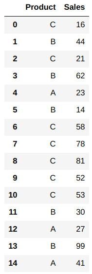
Figure 1.51 – First DataFrame
- Create the second DataFrame similar to how you created the first one. First, create the product lists, as follows:
# Create the second series of products
random.seed(321)
list1 = [['A']*2,['B']*8,['C']*5]
charlist = [x for sublist in list1 for x in sublist]
random.shuffle(charlist)
ser3 = pd.Series(charlist)
ser3
Running this will result in the following output:
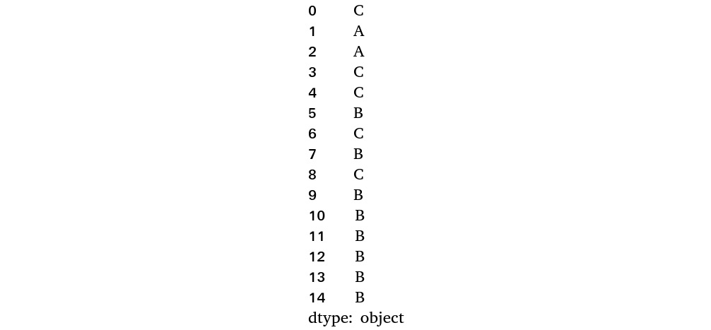
Figure 1.52 – Second DataFrame for products
- Next, create the sales figures:
# Creating sales figures
random.seed(321)
ser4 = pd.Series(random.sample(range(10, 100), 15))
ser4
You should get an output similar to the following:

Figure 1.53 – Series for sales figures
- Finally, create the DataFrame by concatenating both Series (
ser3andser4):# Creating a products data frame prodDf2 = pd.concat([ser3,ser4],axis=1) prodDf2.columns=['Product','Sales'] prodDf2
The output should be as follows:
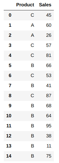
Figure 1.54 – DataFrame created by concatenating ser3 and ser4
- Now, find out how many sales values in the second DataFrame equal
45. This value has been arbitrarily chosen – you may select another value. Do this using thedf.eq()function:prodDf2['Sales'].eq(45)
You should get an output similar to the following:
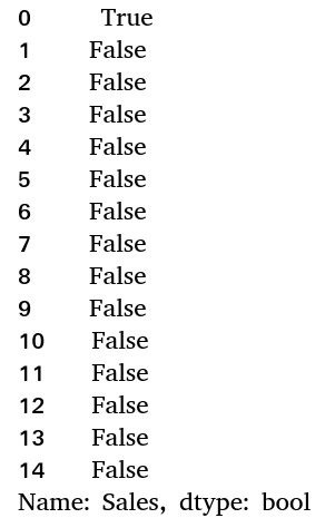
Figure 1.55 – Snapshot of the compared dataset
The output is a Boolean data type. Here, you can see that the first record is where the sales value equals 45. To get only the actual values where the condition has been met and not the Boolean output, subset the DataFrame with the equality comparison within brackets, as follows:
# Comparing values
prodDf2[prodDf2['Sales'].eq(45)]
You should get an output similar to the following:

Figure 1.56 – Records after comparison
From the output, you can see that only the relevant record has been generated.
- Now, verify the number of records where the sales value in the second DataFrame is greater than that in the first one. You can use the
df.gtfunction for this:prodDf2['Sales'].gt(prodDf1['Sales'])
The output will look as follows:
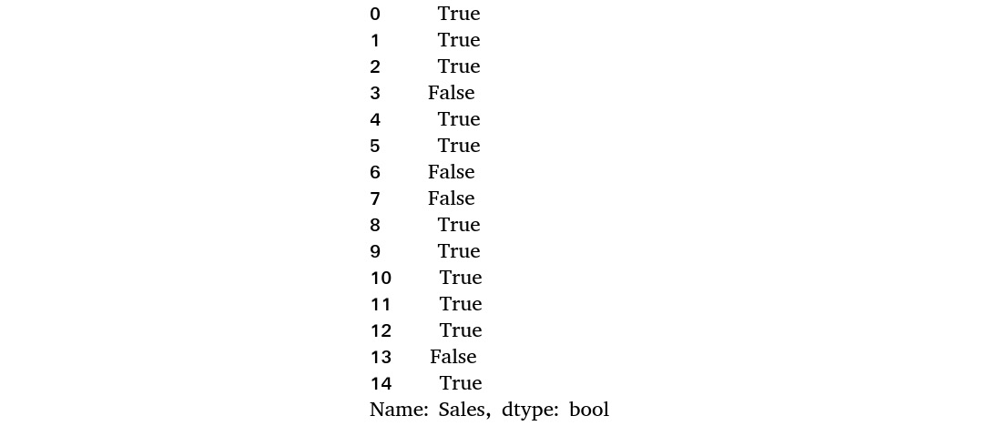
Figure 1.57 – Subset of the DataFrame
- Subset this and find the actual values:
prodDf2[prodDf2['Sales'].gt(prodDf1['Sales'])]
You should get the following output:
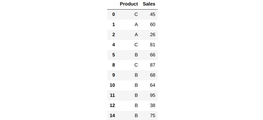
Figure 1.58 – Records after comparison
- Now, implement the
ltfunction to get those rows whereprodDf2is less than the corresponding row ofprodDf1:prodDf2[prodDf2['Sales'].lt(prodDf1['Sales'])]
The output for this should be as follows:

Figure 1.59 – Records after comparison
- Select specific data points from the DataFrame. Use the
df.iloc()method for this, as follows:prodDf2.iloc[[2,5,6,8]]
You should get an output similar to the following:

Figure 1.60 – Accessing records based on their index values
- Now, find the total sales for each product. Then, compare the first DataFrame with the second one by merging both DataFrames based on an overlapping column. Group each DataFrame based on the
Productcolumn and find the total sum of all the values in each group using the aggregate function (.agg()):tab1 = prodDf1.groupby(['Product']).agg('sum') tab2 = prodDf2.groupby(['Product']).agg('sum') print(tab1) print(tab2)
You should get the following output:

Figure 1.61 – Aggregation of products
From the output, you can see that the Sales values for each product have been aggregated.
- Now, merge both DataFrames based on the
Productcolumn:tab3 = pd.DataFrame(pd.merge(tab1,tab2,on=['Product'])) tab3.columns = ['Sales1','Sales2'] tab3
You should get the following output:

Figure 1.62 – Merged DataFrame
The preceding output shows how the sales values, when placed side by side against the corresponding products, help you compare them.
In this exercise, you used some interesting methods to compare two DataFrames and combine two DataFrames based on some overlapping columns. Having learned about these data manipulation methods, it is time to test what you've learned by solving an interesting test case.


