Building a multimodal modular RAG program for drone technology

In the following sections, we will build a multimodal modular RAG-driven generative system from scratch in Python, step by step. We will implement:

• LlamaIndex-managed OpenAI LLMs to process and understand text about drones
• Deep Lake multimodal datasets containing images and labels of drone images taken
• Functions to display images and identify objects within them using bounding boxes
• A system that can answer questions about drone technology using both text and images
• Performance metrics aimed at measuring the accuracy of the modular multimodal responses, including image analysis with GPT-4o

Also, make sure you have created the LLM dataset in Chapter 2 since we will be loading it in this section. However, you can read this chapter without running the notebook since it is self-contained with code and explanations. Now, let’s get to work!

Open the Multimodal_Modular_RAG_Drones.ipynb notebook in the GitHub repository for this chapter at https://github.com/Denis2054/RAG-Driven-Generative-AI/tree/main/Chapter04. The packages installed are the same as those listed in the Installing the environment section of the previous chapter. Each of the following sections will guide you through building the multimodal modular notebook, starting with the LLM module. Let’s go through each section of the notebook step by step.

Loading the LLM dataset

We will load the drone dataset created in Chapter 3. Make sure to insert the path to your dataset:

import deeplake
dataset_path_llm = "hub://denis76/drone_v2"
ds_llm = deeplake.load(dataset_path_llm)

The output will confirm that the dataset is loaded and will display the link to your dataset:

This dataset can be visualized in Jupyter Notebook by ds.visualize() or at https://app.activeloop.ai/denis76/drone_v2
hub://denis76/drone_v2 loaded successfully.

The program now creates a dictionary to hold the data to load it into a pandas DataFrame to visualize it:

import json
import pandas as pd
import numpy as np
# Create a dictionary to hold the data
data_llm = {}
# Iterate through the tensors in the dataset
for tensor_name in ds_llm.tensors:
    tensor_data = ds_llm[tensor_name].numpy()
    # Check if the tensor is multi-dimensional
    if tensor_data.ndim > 1:
        # Flatten multi-dimensional tensors
        data_llm[tensor_name] = [np.array(e).flatten().tolist() for e in tensor_data]
    else:
        # Convert 1D tensors directly to lists and decode text
        if tensor_name == "text":
            data_llm[tensor_name] = [t.tobytes().decode('utf-8') if t else "" for t in tensor_data]
        else:
            data_llm[tensor_name] = tensor_data.tolist()
# Create a Pandas DataFrame from the dictionary
df_llm = pd.DataFrame(data_llm)
df_llm

The output shows the text dataset with its structure: embedding (vectors), id (unique string identifier), metadata (in this case, the source of the data), and text, which contains the content:

Figure 4.2: Output of the text dataset structure and content

We will now initialize the LLM query engine.

Initializing the LLM query engine

As in Chapter 3, Building Indexed-Based RAG with LlamaIndex, Deep Lake, and OpenAI, we will initialize a vector store index from the collection of drone documents (documents_llm) of the dataset (ds). The GPTVectorStoreIndex.from_documents() method creates an index that increases the retrieval speed of documents based on vector similarity:

from llama_index.core import VectorStoreIndex
vector_store_index_llm = VectorStoreIndex.from_documents(documents_llm)

The as_query_engine() method configures this index as a query engine with the specific parameters, as in Chapter 3, for similarity and retrieval depth, allowing the system to answer queries by finding the most relevant documents:

vector_query_engine_llm = vector_store_index_llm.as_query_engine(similarity_top_k=2, temperature=0.1, num_output=1024)

Now, the program introduces the user input.

User input for multimodal modular RAG

The goal of defining the user input in the context of the modular RAG system is to formulate a query that will effectively utilize both the text-based and image-based capabilities. This allows the system to generate a comprehensive and accurate response by leveraging multiple information sources:

user_input="How do drones identify a truck?"

In this context, the user input is the baseline, the starting point, or a standard query used to assess the system’s capabilities. It will establish the initial frame of reference for how well the system can handle and respond to queries utilizing its available resources (e.g., text and image data from various datasets). In this example, the baseline is empirical and will serve to evaluate the system from that reference point.

Querying the textual dataset

We will run the vector query engine request as we did in Chapter 3:

import time
import textwrap
#start the timer
start_time = time.time()
llm_response = vector_query_engine_llm.query(user_input)
# Stop the timer
end_time = time.time()
# Calculate and print the execution time
elapsed_time = end_time - start_time
print(f"Query execution time: {elapsed_time:.4f} seconds")
print(textwrap.fill(str(llm_response), 100))

The execution time is satisfactory:

Query execution time: 1.5489 seconds

The output content is also satisfactory:

Drones can identify a truck using visual detection and tracking methods, which may involve deep neural networks for performance benchmarking.

The program now loads the multimodal drone dataset.

Loading and visualizing the multimodal dataset

We will use the existing pubic VisDrone dataset available on Deep Lake: https://datasets.activeloop.ai/docs/ml/datasets/visdrone-dataset/. We will not create a vector store but simply load the existing dataset in memory:

import deeplake
dataset_path = 'hub://activeloop/visdrone-det-train'
ds = deeplake.load(dataset_path) # Returns a Deep Lake Dataset but does not download data locally

The output will display a link to the online dataset that you can explore with SQL, or natural language processing commands if you prefer, with the tools provided by Deep Lake:

Opening dataset in read-only mode as you don't have write permissions.
This dataset can be visualized in Jupyter Notebook by ds.visualize() or at https://app.activeloop.ai/activeloop/visdrone-det-train
hub://activeloop/visdrone-det-train loaded successfully.

Let’s display the summary to explore the dataset in code:

ds.summary()

The output provides useful information on the structure of the dataset:

Dataset(path='hub://activeloop/visdrone-det-train', read_only=True, tensors=['boxes', 'images', 'labels'])
tensor    htype            shape              dtype     compression
------    -----            -----              -----     -----------
boxes     bbox         (6471, 1:914, 4)       float32          None
images    image        (6471, 360:1500,                            
                        480:2000, 3)          uint8            jpeg
labels    class_label  (6471, 1:914)          uint32           None

The structure contains images, boxes for the boundary boxes of the objects in the image, and labels describing the images and boundary boxes. Let’s visualize the dataset in code:

ds.visualize()

The output shows the images and their boundary boxes:

Figure 4.3: Output showing boundary boxes

Now, let’s go further and display the content of the dataset in a pandas DataFrame to see what the images look like:

import pandas as pd
# Create an empty DataFrame with the defined structure
df = pd.DataFrame(columns=['image', 'boxes', 'labels'])
# Iterate through the samples using enumerate
for i, sample in enumerate(ds):
    # Image data (choose either path or compressed representation)
    # df.loc[i, 'image'] = sample.images.path  # Store image path
    df.loc[i, 'image'] = sample.images.tobytes()  # Store compressed image data
    # Bounding box data (as a list of lists)
    boxes_list = sample.boxes.numpy(aslist=True)
    df.loc[i, 'boxes'] = [box.tolist() for box in boxes_list]
    # Label data (as a list)
    label_data = sample.labels.data()
    df.loc[i, 'labels'] = label_data['text']
df

The output in Figure 4.4 shows the content of the dataset:

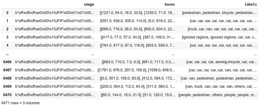
Figure 4.4: Excerpt of the VisDrone dataset

There are 6,471 rows of images in the dataset and 3 columns:

• The image column contains the image. The format of the image in the dataset, as indicated by the byte sequence b'\xff\xd8\xff\xe0\x00\x10JFIF\x00\x01\x01\x00...', is JPEG. The bytes b'\xff\xd8\xff\xe0' specifically signify the start of a JPEG image file.
• The boxes column contains the coordinates and dimensions of bounding boxes in the image, which are normally in the format [x, y, width, height].
• The labels column contains the label of each bounding box in the boxes column.

We can display the list of labels for the images:

labels_list = ds.labels.info['class_names']
labels_list

The output provides the list of labels, which defines the scope of the dataset:

['ignored regions',
 'pedestrian',
 'people',
 'bicycle',
 'car',
 'van',
 'truck',
 'tricycle',
 'awning-tricycle',
 'bus',
 'motor',
 'others']

With that, we have successfully loaded the dataset and will now explore the multimodal dataset structure.

Navigating the multimodal dataset structure

In this section, we will select an image and display it using the dataset’s image column. To this image, we will then add the bounding boxes of a label that we will choose. The program first selects an image.

Selecting and displaying an image

We will select the first image in the dataset:

# choose an image
ind=0
image = ds.images[ind].numpy() # Fetch the first image and return a numpy array

Now, let’s display it with no bounding boxes:

import deeplake
from IPython.display import display
from PIL import Image
import cv2  # Import OpenCV
image = ds.images[0].numpy()
# Convert from BGR to RGB (if necessary)
image_rgb = cv2.cvtColor(image, cv2.COLOR_BGR2RGB)
# Create PIL Image and display
img = Image.fromarray(image_rgb)
display(img)

The image displayed contains trucks, pedestrians, and other types of objects:

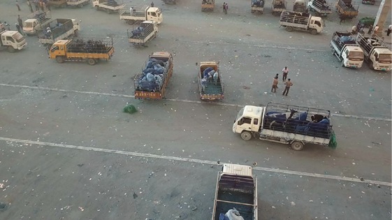
Figure 4.5: Output displaying objects

Now that the image is displayed, the program will add bounding boxes.

Adding bounding boxes and saving the image

We have displayed the first image. The program will then fetch all the labels for the selected image:

labels = ds.labels[ind].data() # Fetch the labels in the selected image
print(labels)

The output displays value, which contains the numerical indices of a label, and text, which contains the corresponding text labels of a label:

{'value': array([1, 1, 7, 1, 1, 1, 1, 6, 6, 6, 6, 6, 6, 6, 6, 6, 6, 1, 6, 6, 6, 6,
       1, 1, 1, 1, 1, 1, 6, 6, 3, 6, 6, 1, 1, 1, 1, 1, 1, 1, 1, 1, 1, 1,
       1, 6, 6, 6], dtype=uint32), 'text': ['pedestrian', 'pedestrian', 'tricycle', 'pedestrian', 'pedestrian', 'pedestrian', 'pedestrian', 'truck', 'truck', 'truck', 'truck', 'truck', 'truck', 'truck', 'truck', 'truck', 'truck', 'pedestrian', 'truck', 'truck', 'truck', 'truck', 'pedestrian', 'pedestrian', 'pedestrian', 'pedestrian', 'pedestrian', 'pedestrian', 'truck', 'truck', 'bicycle', 'truck', 'truck', 'pedestrian', 'pedestrian', 'pedestrian', 'pedestrian', 'pedestrian', 'pedestrian', 'pedestrian', 'pedestrian', 'pedestrian', 'pedestrian', 'pedestrian', 'pedestrian', 'truck', 'truck', 'truck']}

We can display the values and the corresponding text in two columns:

values = labels['value']
text_labels = labels['text']
# Determine the maximum text label length for formatting
max_text_length = max(len(label) for label in text_labels)
# Print the header
print(f"{'Index':<10}{'Label':<{max_text_length + 2}}")
print("-" * (10 + max_text_length + 2))  # Add a separator line
# Print the indices and labels in two columns
for index, label in zip(values, text_labels):
    print(f"{index:<10}{label:<{max_text_length + 2}}")

The output gives us a clear representation of the content of the labels of an image:

Index     Label     
----------------------
1         pedestrian
1         pedestrian
7         tricycle  
1         pedestrian
1         pedestrian
1         pedestrian
1         pedestrian
6         truck     
6         truck    …

We can group the class names (labels in plain text) of the images:

ds.labels[ind].info['class_names'] # class names of the selected image

We can now group and display all the labels that describe the image:

ds.labels[ind].info['class_names'] #class names of the selected image

We can see all the classes the image contains:

['ignored regions',
 'pedestrian',
 'people',
 'bicycle',
 'car',
 'van',
 'truck',
 'tricycle',
 'awning-tricycle',
 'bus',
 'motor',
 'others']

The number of label classes sometimes exceeds what a human eye can see in an image.

Let’s now add bounding boxes. We first create a function to add the bounding boxes, display them, and save the image:

def display_image_with_bboxes(image_data, bboxes, labels, label_name, ind=0):
    #Displays an image with bounding boxes for a specific label.
    image_bytes = io.BytesIO(image_data)
    img = Image.open(image_bytes)
    # Extract class names specifically for the selected image
    class_names = ds.labels[ind].info['class_names']
    # Filter for the specific label (or display all if class names are missing)
    if class_names is not None:
        try:
            label_index = class_names.index(label_name)
            relevant_indices = np.where(labels == label_index)[0]
        except ValueError:
            print(f"Warning: Label '{label_name}' not found. Displaying all boxes.")
            relevant_indices = range(len(labels))
    else:
        relevant_indices = []  # No labels found, so display no boxes
    # Draw bounding boxes
    draw = ImageDraw.Draw(img)
    for idx, box in enumerate(bboxes):  # Enumerate over bboxes
        if idx in relevant_indices:   # Check if this box is relevant
            x1, y1, w, h = box
            x2, y2 = x1 + w, y1 + h
            draw.rectangle([x1, y1, x2, y2], outline="red", width=2)
            draw.text((x1, y1), label_name, fill="red")
    # Save the image
    save_path="boxed_image.jpg"
    img.save(save_path)
    display(img)

We can add the bounding boxes for a specific label. In this case, we selected the "truck" label:

import io
from PIL import ImageDraw
# Fetch labels and image data for the selected image
labels = ds.labels[ind].data()['value']
image_data = ds.images[ind].tobytes()
bboxes = ds.boxes[ind].numpy()
ibox="truck" # class in image
# Display the image with bounding boxes for the label chosen
display_image_with_bboxes(image_data, bboxes, labels, label_name=ibox)

The image displayed now contains the bounding boxes for trucks:

Figure 4.6: Output displaying bounding boxes

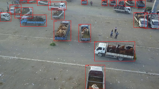
Let’s now activate a query engine to retrieve and obtain a response.

Building a multimodal query engine

In this section, we will query the VisDrone dataset and retrieve an image that fits the user input we entered in the User input for multimodal modular RAG section of this notebook. To achieve this goal, we will:

1. Create a vector index for each row of the df DataFrame containing the images, boxing data, and labels of the VisDrone dataset.
2. Create a query engine that will query the text data of the dataset, retrieve relevant image information, and provide a text response.
3. Parse the nodes of the response to find the keywords related to the user input.
4. Parse the nodes of the response to find the source image.
5. Add the bounding boxes of the source image to the image.
6. Save the image.

Creating a vector index and query engine

The code first creates a document that will be processed to create a vector store index for the multimodal drone dataset. The df DataFrame we created in the Loading and visualizing the multimodal dataset section of the notebook on GitHub does not have unique indices or embeddings. We will create them in memory with LlamaIndex.

The program first assigns a unique ID to the DataFrame:

# The DataFrame is named 'df'
df['doc_id'] = df.index.astype(str)  # Create unique IDs from the row indices

This line adds a new column to the df DataFrame called doc_id. It assigns unique identifiers to each row by converting the DataFrame’s row indices to strings. An empty list named documents is initialized, which we will use to create a vector index:

# Create documents (extract relevant text for each image's labels)
documents = []

Now, the iterrows() method iterates through each row of the DataFrame, generating a sequence of index and row pairs:

for _, row in df.iterrows():
    text_labels = row['labels'] # Each label is now a string
    text = " ".join(text_labels) # Join text labels into a single string
    document = Document(text=text, doc_id=row['doc_id'])
    documents.append(document)

documents is appended with all the records in the dataset, and a DataFrame is created:

# The DataFrame is named 'df'
df['doc_id'] = df.index.astype(str)  # Create unique IDs from the row indices
# Create documents (extract relevant text for each image's labels)
documents = []
for _, row in df.iterrows():
    text_labels = row['labels'] # Each label is now a string
    text = " ".join(text_labels) # Join text labels into a single string
    document = Document(text=text, doc_id=row['doc_id'])
    documents.append(document)

The documents are now ready to be indexed with GPTVectorStoreIndex:

from llama_index.core import GPTVectorStoreIndex
vector_store_index = GPTVectorStoreIndex.from_documents(documents)

The dataset is then seamlessly equipped with indices that we can visualize in the index dictionary:

vector_store_index.index_struct

The output shows that an index has now been added to the dataset:

IndexDict(index_id='4ec313b4-9a1a-41df-a3d8-a4fe5ff6022c', summary=None, nodes_dict={'5e547c1d-0d65-4de6-b33e-a101665751e6': '5e547c1d-0d65-4de6-b33e-a101665751e6', '05f73182-37ed-4567-a855-4ff9e8ae5b8c': '05f73182-37ed-4567-a855-4ff9e8ae5b8c'

We can now run a query on the multimodal dataset.

Running a query on the VisDrone multimodal dataset

We now set vector_store_index as the query engine, as we did in the Vector store index query engine section in Chapter 3:

vector_query_engine = vector_store_index.as_query_engine(similarity_top_k=1, temperature=0.1, num_output=1024)

We can also run a query on the dataset of drone images, just as we did in Chapter 3 on an LLM dataset:

import time
start_time = time.time()
response = vector_query_engine.query(user_input)
# Stop the timer
end_time = time.time()
# Calculate and print the execution time
elapsed_time = end_time - start_time
print(f"Query execution time: {elapsed_time:.4f} seconds")

The execution time is satisfactory:

Query execution time: 1.8461 seconds

We will now examine the text response:

print(textwrap.fill(str(response), 100))

We can see that the output is logical and therefore satisfactory.

Drones use various sensors such as cameras, LiDAR, and GPS to identify and track objects like trucks.

Processing the response

We will now parse the nodes in the response to find the unique words in the response and select one for this notebook:

from itertools import groupby
def get_unique_words(text):
    text = text.lower().strip()
    words = text.split()
    unique_words = [word for word, _ in groupby(sorted(words))]
    return unique_words
for node in response.source_nodes:
    print(node.node_id)
    # Get unique words from the node text:
    node_text = node.get_text()
    unique_words = get_unique_words(node_text)
    print("Unique Words in Node Text:", unique_words)

We found a unique word ('truck') and its unique index, which will lead us directly to the image of the source of the node that generated the response:

1af106df-c5a6-4f48-ac17-f953dffd2402
Unique Words in Node Text: ['truck']

We could select more words and design this function in many different ways depending on the specifications of each project.

We will now search for the image by going through the source nodes, just as we did for an LLM dataset in the Query response and source section of the previous chapter. Multimodal vector stores and querying frameworks are flexible. Once we learn how to perform retrievals on an LLM and a multimodal dataset, we are ready for anything that comes up!

Let’s select and process the information related to an image.

Selecting and processing the image of the source node

Before running the image retrieval and displaying function, let’s first delete the image we displayed in the Adding bounding boxes and saving the image section of this notebook to make sure we are working on a new image:

# deleting any image previously saved
!rm /content/boxed_image.jpg

We are now ready to search for the source image, call the bounding box, and display and save the function we defined earlier:

display_image_with_bboxes(image_data, bboxes, labels, label_name=ibox)

The program now goes through the source nodes with the keyword "truck" search, applies the bounding boxes, and displays and saves the image:

import io
from PIL import Image
def process_and_display(response, df, ds, unique_words):
    """Processes nodes, finds corresponding images in dataset, and displays them with bounding boxes.
    Args:
        response: The response object containing source nodes.
        df: The DataFrame with doc_id information.
        ds: The dataset containing images, labels, and boxes.
        unique_words: The list of unique words for filtering.
    """
…
            if i == row_index:
                image_bytes = io.BytesIO(sample.images.tobytes())
                img = Image.open(image_bytes)
                labels = ds.labels[i].data()['value']
                image_data = ds.images[i].tobytes()
                bboxes = ds.boxes[i].numpy()
                ibox = unique_words[0]  # class in image
                display_image_with_bboxes(image_data, bboxes, labels, label_name=ibox)
# Assuming you have your 'response', 'df', 'ds', and 'unique_words' objects prepared:
process_and_display(response, df, ds, unique_words)

The output is satisfactory:

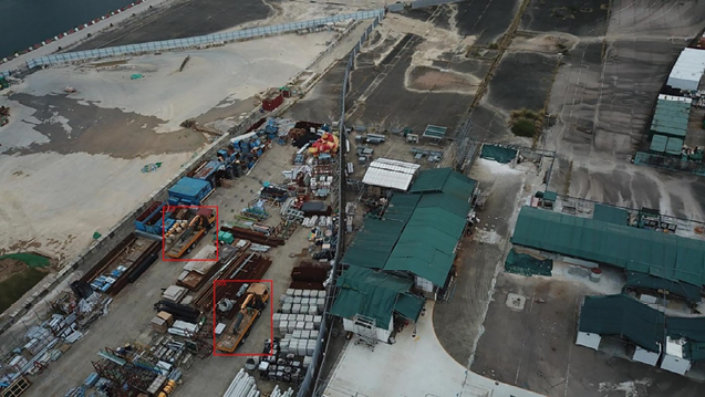
Figure 4.7: Displayed satisfactory output

Multimodal modular summary

We have built a multimodal modular program step by step that we can now assemble in a summary. We will create a function to display the source image of the response to the user input, then print the user input and the LLM output, and display the image.

First, we create a function to display the source image saved by the multimodal retrieval engine:

# 1.user input=user_input
print(user_input)
# 2.LLM response
print(textwrap.fill(str(llm_response), 100))
# 3.Multimodal response
image_path = "/content/boxed_image.jpg"
display_source_image(image_path)

Then, we can display the user input, the LLM response, and the multimodal response. The output first displays the textual responses (user input and LLM response):

How do drones identify a truck?
Drones can identify a truck using visual detection and tracking methods, which may involve deep neural networks for performance benchmarking.

Then, the image is displayed with the bounding boxes for trucks in this case:

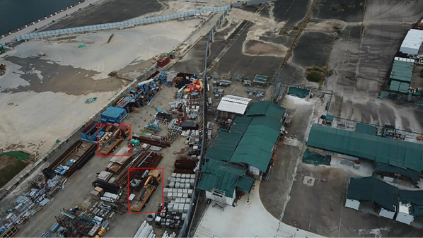
Figure 4.8: Output displaying boundary boxes

By adding an image to a classical LLM response, we augmented the output. Multimodal RAG output augmentation will enrich generative AI by adding information to both the input and output. However, as for all AI programs, designing a performance metric requires efficient image recognition functionality.

Performance metric

Measuring the performance of a multimodal modular RAG requires two types of measurements: text and image. Measuring text is straightforward. However, measuring images is quite a challenge. Analyzing the image of a multimodal response is quite different. We extracted a keyword from the multimodal query engine. We then parsed the response for a source image to display. However, we will need to build an innovative approach to evaluate the source image of the response. Let’s begin with the LLM performance.

LLM performance metric

LlamaIndex seamlessly called an OpenAI model through its query engine, such as GPT-4, for example, and provided text content in its response. For text responses, we will use the same cosine similarity metric as in the Evaluating the output with cosine similarity section in Chapter 2, and the Vector store index query engine section in Chapter 3.

The evaluation function uses sklearn and sentence_transformers to evaluate the similarity between two texts—in this case, an input and an output:

from sklearn.feature_extraction.text import TfidfVectorizer
from sklearn.metrics.pairwise import cosine_similarity
from sentence_transformers import SentenceTransformer
model = SentenceTransformer('all-MiniLM-L6-v2')
def calculate_cosine_similarity_with_embeddings(text1, text2):
    embeddings1 = model.encode(text1)
    embeddings2 = model.encode(text2)
    similarity = cosine_similarity([embeddings1], [embeddings2])
    return similarity[0][0]

We can now calculate the similarity between our baseline user input and the initial LLM response obtained:

llm_similarity_score = calculate_cosine_similarity_with_embeddings(user_input, str(llm_response))
print(user_input)
print(llm_response)
print(f"Cosine Similarity Score: {llm_similarity_score:.3f}")

The output displays the user input, the text response, and the cosine similarity between the two texts:

How do drones identify a truck?
How do drones identify a truck?
Drones can identify a truck using visual detection and tracking methods, which may involve deep neural networks for performance benchmarking.
Cosine Similarity Score: 0.691

The output is satisfactory. But we now need to design a way to measure the multimodal performance.

Multimodal performance metric

To evaluate the image returned, we cannot simply rely on the labels in the dataset. For small datasets, we can manually check the image, but when a system scales, automation is required. In this section, we will use the computer vision features of GPT-4o to analyze an image, parse it to find the objects we are looking for, and provide a description of that image. Then, we will apply cosine similarity to the description provided by GPT-4o and the label it is supposed to contain. GPT-4o is a multimodal generative AI model.

Let’s first encode the image to simplify data transmission to GPT-4o. Base64 encoding converts binary data (like images) into ASCII characters, which are standard text characters. This transformation is crucial because it ensures that the image data can be transmitted over protocols (like HTTP) that are designed to handle text data smoothly. It also avoids issues related to binary data transmission, such as data corruption or interpretation errors.

The program encodes the source image using Python’s base64 module:

import base64
IMAGE_PATH = "/content/boxed_image.jpg"
# Open the image file and encode it as a base64 string
def encode_image(image_path):
    with open(image_path, "rb") as image_file:
        return base64.b64encode(image_file.read()).decode("utf-8")
base64_image = encode_image(IMAGE_PATH)

We now create an OpenAI client and set the model to gpt-4o:

from openai import OpenAI
#Set the API key for the client
client = OpenAI(api_key=openai.api_key)
MODEL="gpt-4o"

The unique word will be the result of the LLM query to the multimodal dataset we obtained by parsing the response:

u_word=unique_words[0]
print(u_word)

We can now submit the image to OpenAI GPT-4o:

response = client.chat.completions.create(
    model=MODEL,
    messages=[
        {"role": "system", "content": f"You are a helpful assistant that analyzes images that contain {u_word}."},
        {"role": "user", "content": [
            {"type": "text", "text": f"Analyze the following image, tell me if there is one {u_word} or more in the bounding boxes and analyze them:"},
            {"type": "image_url", "image_url": {
                "url": f"data:image/png;base64,{base64_image}"}
            }
        ]}
    ],
    temperature=0.0,
)
response_image = response.choices[0].message.content
print(response_image)

We instructed the system and user roles to analyze images looking for our target label, u_word—in this case, truck. We then submitted the source node image to the model. The output that describes the image is satisfactory:

The image contains two trucks within the bounding boxes. Here is the analysis of each truck:
1. **First Truck (Top Bounding Box)**:
   - The truck appears to be a flatbed truck.
   - It is loaded with various materials, possibly construction or industrial supplies.
   - The truck is parked in an area with other construction materials and equipment.
2. **Second Truck (Bottom Bounding Box)**:
   - This truck also appears to be a flatbed truck.
   - It is carrying different types of materials, similar to the first truck.
   - The truck is situated in a similar environment, surrounded by construction materials and equipment.
Both trucks are in a construction or industrial area, likely used for transporting materials and equipment.

We can now submit this response to the cosine similarity function by first adding an "s" to align with multiple trucks in a response:

resp=u_word+"s"
multimodal_similarity_score = calculate_cosine_similarity_with_embeddings(resp, str(response_image))
print(f"Cosine Similarity Score: {multimodal_similarity_score:.3f}")

The output describes the image well but contains many other descriptions beyond the word “truck,” which limits its similarity to the input requested:

Cosine Similarity Score: 0.505

A human observer might approve the image and the LLM response. However, even if the score was very high, the issue would be the same. Complex images are challenging to analyze in detail and with precision, although progress is continually made. Let’s now calculate the overall performance of the system.

Multimodal modular RAG performance metric

To obtain the overall performance of the system, we will divide the sum of the LLM response and the two multimodal response performances by 2:

score=(llm_similarity_score+multimodal_similarity_score)/2
print(f"Multimodal, Modular Score: {score:.3f}")

The result shows that although a human who observes the results may be satisfied, it remains difficult to automatically assess the relevance of a complex image:

Multimodal, Modular Score: 0.598

The metric can be improved because a human observer sees that the image is relevant. This explains why the top AI agents, such as ChatGPT, Gemini, and Bing Copilot, always have a feedback process that includes thumbs up and thumbs down.

Let’s now sum up the chapter and gear up to explore how RAG can be improved even further with human feedback.